![]() ISSN 0798 1015
ISSN 0798 1015

![]() ISSN 0798 1015
ISSN 0798 1015
Vol. 41 (Issue 01) Year 2020. Page 18
NUGRAHADI, Eko Wahyu 1; MAIPITA, Indra 2 & SITUMEANG, Chandra 3
Received: 29/08/2019 • Approved: 11/01/2020 • Published 15/01/20
ABSTRACT: This study aims to analyze the dominant factors that affect the optimal performance of the economic policy of the small business sector with case study in food, beverage and tobacco sector development in North Sumatra, Indonesia. Using Principal Component Analysis [PCA], the components examined are investment, wage, inflation, exchange rate, population, total workers, GDRP, industrial GDRP, interest rate and total credit. The results of the analysis show that the variables which are the two dominant factors are population and credit. |
RESUMEN: Este estudio tiene como objetivo analizar los factores dominantes que afectan el desempeño óptimo de la política económica del sector de pequeñas empresas con estudios de caso en el desarrollo del sector de alimentos, bebidas y tabaco en el norte de Sumatra, Indonesia. Utilizando el análisis de componentes principales [PCA], los componentes examinados son inversión, salario, inflación, tipo de cambio, población, trabajadores totales, GDRP, GDRP industrial, tasa de interés y crédito total. Los resultados del análisis muestran que las variables que son los dos factores dominantes son la población y el crédito. |

The achievement of high economic growth is the main target that will normally be pursued in an economy in order to realize a just and prosperous society. North Sumatra's economic growth as measured by Gross Regional Domestic Product (GRDP) based on constant prices in 2000, from 2010 to 2014 experienced a significant increase (Figure 1). In average during 5 years, the growth of North Sumatra was 6.11%. This indicates that the welfare of the people of North Sumatra is increasing. Especially when it is related to the condition of the number of poor people in this area within this period decreased from 11.31% (2010) to 10.39% (2013).
During the period 2010-2014 the development of the North Sumatra Gini Ratio Index has increased (from 0.350 in 2010 to 0.354 in 2014) so that income inequality between households in North Sumatra tends to increase. Also, the Gini Ratio indicates that during this period the condition of income inequality between households was relatively high. Thus the high economic growth of North Sumatra and the tendency to increase are not fully enjoyed by all levels of society, thus leading to the creation of income gaps between households and poverty. Thus the size of the outcome of economic development cannot only be reflected by the high economic growth and the amount of regional income, but also includes among the following things related to human development: income inequality, the number of poor and unemployed. Therefore, in designing an economic development strategy so that it is not only aimed at economic growth (growth), but also needs to be followed by an improvement in addition to the decline in the number of poor people, reduce unemployment and regarding income distribution. The question needs further analysis to get more in-depth information in the sectoral development of Small Food, Beverage and Tobacco industry. This study aims to analyze the dominant factors that influence the optimal performance of the economic policy of the Small business sector of food, beverage and tobacco industrial sector development.
Figure 1
Gross Regional Domestic Product of
North Sumatra (in billions of Rupiah)
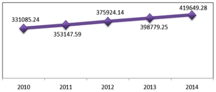
(Source: BPS, 2010-2014)
This study uses Structural Equation Modeling analysis, also called Linear Structural Relationships (LISREL) or analysis of covariance structure. This method is used to analyze microeconomic aspects focussing to find out the dominant factors that influence the performance of optimal sectoral development economic policies. Before testing the factor analysis, assumption testing is carried out, namely the nominality test and the multicollinearity test.
1) Normality Test
This test aims to see whether the sample is normally distributed or not. The test used is the normality test on the non-parametric sample Kolmogrov Smirnov with the following criteria:
If Significance (Sig.) or probability <0.05 then the sample is normally distributed.
If Significant or probability> 0.05 then the sample is not normally distributed.
(Santoso, 2008)
2) Multicollinearity Test
Unlike the regression analysis which tends to avoid multicollinearity, factor analysis is the opposite. In this study, multicollinearity is expected to occur as a basis for the formation of new factors as a combination of several variables that are collinear. This can be done with the Kaiser Meyer Olki (KMO) test with the criteria if the KMO Adequancy value is greater than 0.5, multicollinearity occurs in the research variables making it feasible to test further factor analysis.
To answer a hypothesis that is a dominant indicator or variable, it is necessary to extract many of these variables into several parts. However, because the research data used are generally large amounts of ratio data (thousands, millions, billions), it is necessary to simplify the form through data transformation using logarithms. To extract many variables, the analysis method used in this research is factor analysis. Factor analysis is principally used to reduce data, which is the process of summarizing a number of variables to be smaller and calling them factor analysis.
Stages in factor analysis:
1. Select variables that are feasible in factor analysis. Because factor analysis seeks to group a number of variables, there should be a strong enough correlation between variables so that grouping will occur. If a variable or more is weakly correlated with other variables, then that variable will be excluded from factor analysis.
2. After a number of variables are selected, extraction of the variable is carried out to become one or several factors. Some popular factor search methods are Principal Components and Maximum Likehood.
3. The factors formed, in many cases, do not adequately reflect the differences between the factors that exist. After the factors are formed, the process is continued by naming the factors that exist.
All factor analysis calculations in this study were carried out using Software Statistical Product Social Science (SPSS) 18 for windows. And the data used are secondary data with the type of time series data (time series) during the period (1995-2015). With data used sourced from the Central Statistics Agency (BPS) and Bank Indonesia (BI). The data needed is North Sumatra data which includes: investment, investment in the previous year, UMR, inflation, exchange rate, population, number of workers in the Small IMMT industry, GRDP, GRDP in the industrial sector, loan interest rates and total credit.
Principal component analysis [PCA] is used to determine whether research is feasible to be used for factor analysis or factor analysis. For this, the Kaiser Meyer Olkin [KMO] value and Bartlet test are used. PCA is a technique for shrinking data where the main goal is to reduce the number of dimensions of correlated variables into new variables, called principal components or principal components, which do not correlate by maintaining as much diversity as possible in the data set.
Factor analysis will produce communalities analysis. Communalities analysis is basically the amount of variance in the form of a percentage of each initial variable that can be explained by existing factors.
After one or more factors are formed, with a factor containing a number of variables obtained through the main component method. In general, these factors are difficult to interpret directly or it is difficult for those variables to be determined which factors to enter. Or if only one factor is formed from the factoring process, then a variable may be doubted whether it is feasible or not included in the factor formed. To overcome this it can be done by a rotation process on the factors formed, so as to clarify the position of a variable, whether included in one factor or included in another factor. This is usually called factor rotation.
The method of rotation of the factors used in this study uses the Varimax orthogonal rotation method. Varimax is rotation which maximizes the weighting and results in the correlation of variables with a factor approaching one and the correlation with other factors approaching zero.
The result of this rotation factor is an attempt to produce a new weighing factor that is more easily interpreted, namely by multiplying the original weighing factor with a transformation matrix that is orthogonal so that the correlation matrix does not change. From rotation matrix loading it is shown that each variable that has a high correlation> 0.05 will be included in a particular factor, while other variables that have a low correlation <0.05, then it will not be included in certain factors or ignored. So in the end every variable and factor formed will be more easily interpreted.
Furthermore, to test the hypotheses proposed in this study, namely that there is the most dominant indicator in the large medium industry in the food and beverage and tobacco sectors, and then it can be done by sorting the factor scores from the largest to the smallest values. The ways to find out the factor scores are:
Furthermore, the results obtained from the calculation of the factor score and to determine the most dominant factor can be done by knowing the largest factor score.
Normality testing can be done with non-parametric sample Kolmogrov Smirnov, where to find out normal data or not indicated by criteria if the Sig. > 0.05 then the data is normal. Table 1. shows the results of the calculation of the value of Sig. of the 11 variables defined in this study. From table 1 it is shown that all Sig. as a whole> 0.05, it can be concluded that all data are normally distributed.
Table 1
Normality Testing with Kolmogorov
Smirnov One-Sample
Variable |
Initial |
Investment |
0.763 |
Investment t-1 |
0.700 |
Local minimum wage |
0.992 |
Inflation |
0.400 |
Exchange rate |
0.400 |
Population |
0.883 |
Total workers |
0.504 |
GDRP |
0.988 |
Industrial GDRP |
0.977 |
Interest rate |
0.948 |
Total credit |
0.987 |
In contrast to the regression analysis which tends to avoid multicollinearity, in this study multicollinearity is expected to be the basis for the formation of new factors as a combination of several collinearity variables analyzed by the KMO Test and the Barlett's Test. This test is intended to determine whether the overall factor analysis variable is feasible for further factor analysis with the criteria that if the KMO MSA value> 0.5, and the Sig. Bartlett's Test <0.05, the overall variables used are eligible for further analysis. The results of the KMO multicollinearity test and Bartlett's Test of this study are in Table 2.
Table 2
KMO and Bartlett's Test
Kaiser-Meyer-Olkin Measure of Sampling Adequacy |
.762 |
|
Bartlett's Test of Sphericity |
Approx. Chi-Square |
322.584 |
df |
55 |
|
Sig. |
.000 |
|
Based on Table 2, there are two known ways to test multicollinearity. (a) The Kaiser-Meyer-Olkin Test (KMO), that can find out the KMO Adequacy value of 0.762 which is > 0.5. Thus all the factors of this factor analysis can be processed further. (b) Bartlett's test, that can be known the Chi Square value of 322.584 with a significance of 0.000 which is <0.05, meaning that there is a significant correlation between the overall factor analysis variables. Thus, overall, all the variables of the analysis of this factor analysis can be done with a factor analysis test.
However, to find out more about any variable in this factor analysis it is necessary to do further anti image matrices test.
Anti Image Matrices - Measure of Sampling Adequacy (MSA) Test is to find out which variables are feasible and not feasible to be used in further factor analysis. The MSA rate ranges from 0 to 1, with the following criteria:
• MSA = 1, meaning that the variable can be predicted without error by other variables.
• MSA> 0.5, meaning that variables can still be predicted and can be further analyzed.
• MSA <0.5, meaning that the variable cannot be predicted and cannot be further analyzed, or excluded from other variables.
So from this basis to assess which variables are worth further use in this factor analysis research.
The results of the anti-image matrices correlation test of this study are in Table 3.
Table 3
Anti Image
Matrices Correlation
|
X1 |
X2 |
X3 |
X4 |
X5 |
X6 |
X7 |
X8 |
X9 |
X10 |
X11 |
|
Anti-image Correlation |
Investment |
.797a |
-.486 |
-.424 |
-.534 |
-.138 |
-.300 |
.280 |
-.267 |
-.197 |
.407 |
.609 |
Investment t-1 |
-.486 |
.835a |
.345 |
.477 |
.110 |
-.005 |
-.364 |
.157 |
.312 |
-.259 |
-.562 |
|
Local minimum wage |
-.424 |
.345 |
.740a |
.173 |
.773 |
-.184 |
-.196 |
-.360 |
.582 |
-.757 |
-.720 |
|
Inflation |
-.534 |
.477 |
.173 |
.548a |
-.195 |
.550 |
-.030 |
.579 |
-.241 |
-.459 |
-.448 |
|
Exchange rate |
-.138 |
.110 |
.773 |
-.195 |
.559a |
-.446 |
-.149 |
-.676 |
.725 |
-.655 |
-.472 |
|
Population |
-.300 |
-.005 |
-.184 |
.550 |
-.446 |
.847a |
.090 |
.582 |
-.556 |
-.197 |
-.078 |
|
Total workers |
.280 |
-.364 |
-.196 |
-.030 |
-.149 |
.090 |
.853a |
-.271 |
-.561 |
-.050 |
.668 |
|
GDRP |
-.267 |
.157 |
-.360 |
.579 |
-.676 |
.582 |
-.271 |
.810a |
-.543 |
.198 |
-.162 |
|
Industrial GDRP |
-.197 |
.312 |
.582 |
-.241 |
.725 |
-.556 |
-.561 |
-.543 |
.759a |
-.233 |
-.610 |
|
Interest rate |
.407 |
-.259 |
-.757 |
-.459 |
-.655 |
-.197 |
-.050 |
.198 |
-.233 |
.743a |
.565 |
|
Total credit |
.609 |
-.562 |
-.720 |
-.448 |
-.472 |
-.078 |
.668 |
-.162 |
-.610 |
.565 |
.727a |
|
The testing results from KMO test and Bartlett’s Test and Anti Image Correlation test are intended to determine whether the overall factor analysis variable is suitable for further factor analysis. By using the criteria KMO MSA significant value> 0.5, and the significant value of Bartlett's Test <0.05, the results showed that overall variables used are eligible for further analysis.
Communalities analysis is basically the amount of variance in the form of a percentage of each initial variable that can be explained by existing factors. The variable values in the communalities table with Extraction > 0.5, explain that the variables used have a strong relationship with the factors that are formed. In other words, the greater the value of the communalities, the better the factor analysis, because the greater the characteristics of the original variable that can be represented by the factors formed. Table 4 shows that the relationship of the investment variable to the factor is closely formed (81.4 percent, and the contribution of the previous year's investment variable to the factors formed was 82.5 percent. Moreover, the relationship between the local minimum wage variables and the factors that are formed is very close (95.5 percent), and the relationship of the inflation variable to the factor is closely formed (84.6 percent). Furthermore, the exchange rate variable relationship to the factors that are closely formed (82.9 percent), and the relationship of the variable of the population to the factors that are formed is very close ( 97 percent).
Table 4
Communalities
Variable |
Initial |
Extraction |
Investment |
1.000 |
.814 |
Investment t-1 |
1.000 |
.825 |
Local minimum wage |
1.000 |
.955 |
Inflation |
1.000 |
.846 |
Exchange rate |
1.000 |
.829 |
Population |
1.000 |
.970 |
Total workers |
1.000 |
.860 |
GDRP |
1.000 |
.988 |
Industrial GDRP |
1.000 |
.982 |
Interest rate |
1.000 |
.890 |
Total credit |
1.000 |
.975 |
Extraction Method: Principal Component Analysis |
||
The relationship between the variables of labor and factors is 86 percent, and the relationship between the GDP variable to the factors that are formed is 98.8 percent. Moreover, the relationship between the industrial sector GDP variables to the factors that are very closely formed (98.2 percent), and the relationship between loan interest rates and closely formed factors (89 percent), In terms of the relationship between the total loan variables, it has value of 97.5 percent. According;y, the overall variance value of the variables in this study shows a large enough value> 0.5, so that factor analysis can be carried out without removing the variables in this study. From the communalities analysis it is stated that there are 11 variables that can be forwarded for factor analysis, so there will be 11 components or 11 initial factors that will be used in factor analysis. Next step is to determine how many factors might be formed which can be explained in the Total Variance Explained.
Table 5 shows the ability of each factor to explain or represent research variables, indicated by the variance explained or initial eigenvalue. Components or factors that will be selected are factors with eigenvalue values greater than 1, where only the factors that are able to explain the variables well. Of the 11 components, only 2 factors were formed because the eigenvalue value was greater than 1. While the other 9 factors were not included in the factor analysis because they were unable to explain the variables properly. In the extraction sums of squared loadings column, there is a% of variance column that shows the percentage of variance that can be explained by factors, while cumulative percent is the percentage of variance explained by each factor. Of the 2 factors that are formed will be able to explain the variance in total by 90.31 percent variables. If there is only 1 factor (the first factor), it can only explain the total variable variance of 79.23 percent.
Table 5
Total Variance Explained
Component |
Initial Eigenvalues |
Extraction Sums of Squared Loadings |
Rotation Sums of Squared Loadings |
||||||
Total |
% of Variance |
Cumulative % |
Total |
% of Variance |
Cumulative % |
Total |
% of Variance |
Cumulative % |
|
1 |
8.716 |
79.235 |
79.235 |
8.716 |
79.235 |
79.235 |
7.154 |
65.036 |
65.036 |
2 |
1.218 |
11.075 |
90.310 |
1.218 |
11.075 |
90.310 |
2.780 |
25.274 |
90.310 |
3 |
.445 |
4.049 |
94.359 |
- |
- |
- |
- |
- |
- |
4 |
.215 |
1.952 |
96.311 |
- |
- |
- |
- |
- |
- |
5 |
.193 |
1.753 |
98.063 |
- |
- |
- |
- |
- |
- |
6 |
.105 |
.958 |
99.021 |
- |
- |
- |
- |
- |
- |
7 |
.079 |
.723 |
99.744 |
- |
- |
- |
- |
- |
- |
8 |
.023 |
.209 |
99.952 |
- |
- |
- |
- |
- |
- |
9 |
.004 |
.037 |
99.990 |
- |
- |
- |
- |
- |
- |
10 |
.001 |
.007 |
99.996 |
- |
- |
- |
- |
- |
- |
11 |
.000 |
.004 |
100.000 |
- |
- |
- |
- |
- |
- |
Extraction Method: Principal Component Analysis. |
|||||||||
After removing the factor that has eigenvalue less than 1 then there will only be 2 new factors formed in factor analysis. Component matrix there will be 2 component columns. The values contained in the column indicate the loading factor, where the loading factor shows the correlation between one variable and the selected factor. A large factor loading value indicates that the variable is included in the component of the formed factor.
Table 6 shows that the variable correlation value is still very evenly distributed, where the magnitude of the correlation of a variable in one component of the factor is still relatively the same as the magnitude of the variable correlation on other factors . For this reason rotation is carried out on the factor dimension, so that the rotated component matrix is obtained. Rotation is done by the varimax method, where varimax rotation is chosen because it is easier to analyze in theory.
Table 6
Component Matrix
|
Component |
|
1 |
2 |
|
Investment |
.895 |
.114 |
Investment t-1 |
.908 |
-.010 |
Local minimum wage |
.974 |
.084 |
Inflation |
-.510 |
.765 |
Exchange rate |
.646 |
.642 |
Population |
.976 |
.134 |
Total workers |
.924 |
-.078 |
GDRP |
.994 |
.022 |
Industrial GDRP |
.991 |
.014 |
Interest rate |
-.847 |
.416 |
Total credit |
.985 |
.062 |
Extraction Method: Principal Component Analysis. |
||
a. 2 components extracted. |
||
-----
Table 7
Rotated Component Matrix
|
Component |
|
1 |
2 |
|
Investment |
.848 |
.307 |
Investment t-1 |
.803 |
.424 |
Local minimum wage |
.905 |
.370 |
Inflation |
-.105 |
-.914 |
Exchange rate |
.868 |
-.276 |
Population |
.929 |
.327 |
Total workers |
.786 |
.492 |
GDRP |
.894 |
.434 |
Industrial GDRP |
.888 |
.440 |
Interest rate |
-.564 |
-.756 |
Total credit |
.905 |
.395 |
Extraction Method: Principal Component Analysis. Rotation Method: Varimax with Kaiser Normalization. |
||
a. Rotation converged in 3 iterations. |
||
Table 7 shows the value of the correlation of a dominant variable in the new factor component that is formed. Determination of variables that enter the new factor component based on correlation values greater than 0.5. For example, the investment variable that enters the component factor 1 with a factor loading of 0.848. Specifically the value of the factor loading variable of the loan interest rate is both> 0.5, then it is determined by which factor loading factor is the biggest, which is grouped in factor 2 with a value of 0.756. Furthermore, based on the results of the calculation can be grouped variables into newly formed factors. Following are groups of variables in these factors:
Factor 1: Investment, investment in the previous year, local minimum wage, exchange rate, total population, labor, Grdp, industrial GRDP, and total credit.
Factor 2: Inflation and loan interest rates.
As the last step is to find out the accuracy of the factors formed from all the factor analysis variables used by using the Component Transformation Matrix.
Table 8
Component Tranformation Matrix
Component |
Factor 1 |
Factor 2 |
Factor 1 |
.890 |
.456 |
Factor 2 |
.456 |
-.890 |
Extraction Method: Principal Component Analysis. Rotation Method: Varimax with Kaiser Normalization. |
||
Table 8 shows that either the component factor 1 or factor 2 has a correlation of 0.890 which means it has a strong correlation because 0.890> 0.5. Thus, it is known that the factor 1 and factor 2 formed can be said to be appropriate to summarize the 11 independent variables used in factor analysis in this study.
Table 9 shows three dominant factors in the food, beverage and tobacco industry, namely the population, total credit and local minimum wage. Table 9 also shows that the population is the most dominant indicator in small business sector of food, beverage and tobacco. This can be understood, because one of the factors that influence demand is the population or number of consumers. The large number of people in North Sumatra can be an opportunity for small business sector of food, beverage and tobacco market share. The large number of people in an area will have an impact on increasing needs, especially in food and beverages. This is a good opportunity for businesses to meet the growing market demand. So it is very reasonable if the population is the most dominant factor affecting the development of small business sector of food, beverage and tobacco in North Sumatra Province. However, the most interesting thing in this study is the second dominant factor, namely the amount of credit.
Table 9
Dominant Indicators
No |
Variable |
Rotated Component Matrix |
Variance |
Total Variance |
Factor Score |
Indicator Sequences |
||
Factor 1 |
Factor 2 |
|||||||
1 |
2 |
8.716 |
1.218 |
9.934 |
||||
1 |
investment |
0.848 |
0.307 |
7.391 |
0.374 |
7.765 |
0.782 |
6 |
2 |
investment t-1 |
0.803 |
0.424 |
6.999 |
0.516 |
7.515 |
0.757 |
7 |
3 |
local minimum wage |
0.905 |
0.370 |
7.888 |
0.451 |
8.339 |
0.839 |
3 |
4 |
inflation |
-0.105 |
-0.914 |
-0.915 |
-1.113 |
-2.028 |
-0.204 |
11 |
5 |
exchange rate |
0.868 |
-0.276 |
7.565 |
-0.336 |
7.229 |
0.728 |
9 |
6 |
population |
0.929 |
0.327 |
8.097 |
0.398 |
8.495 |
0.855 |
1 |
7 |
total labor |
0.786 |
0.492 |
6.851 |
0.599 |
7.450 |
0.750 |
8 |
8 |
GDRP |
0.894 |
0.434 |
7.792 |
0.529 |
8.321 |
0.838 |
4 |
9 |
industrial GDRP |
0.888 |
0.440 |
7.740 |
0.536 |
8.276 |
0.833 |
5 |
10 |
interest rate |
-0.564 |
-0.756 |
-4.916 |
-0.921 |
-5.837 |
-0.588 |
10 |
11 |
total credit |
0.905 |
0.395 |
7.888 |
0.481 |
8.369 |
0.842 |
2 |
The results of this study explained that the amount of credit was dominant in determining the development of the small business sectors of food, beverage and tobacco in North Sumatra. When linked to the amount of credit, what needs more special attention is the performance of banks in channeling credit in North Sumatra. The banking industry has an important role in the economy as an intermediary institution that distributes public funds into productive asset investments that will encourage real sector productivity, capital accumulation, and aggregate output growth (Bencivenga and Smith, 1991; Hung and Cothern, 2002). For analysis at the country level, King and Levine (1993), Levine (1998) and Rajan and Zingales (1998) provide support for the positive impact of bank credit on per capita income growth, both in developed and developing countries. Separately, Demirgüç-Kunt and Maksimovic (2002) in their study showed that credit recipient companies tend to experience increased income. On the other hand, previous studies also show that bank credit does not always encourage economic growth. The positive influence of bank credit on the economy will only occur, if the fundamental quality in a country, such as physical capital (gross capital formation) or the quality of infrastructure has reached a certain level sufficient to encourage productivity and competency of the real sector (Augier and Soedarmono, 2011; Meslier-Crouzille et al., 2012; Deidda and Fattouh, 2002). Furthermore, Meslier-Crouzille et al. (2012) further explained that the positive relationship between the financial sector and economic growth is only seen in countries with a level of development that has reached a fairly good level. At the individual bank level, banks will encourage optimal financial intermediation by providing more competitive loan interest rates, if bank management has achieved a certain level of cost-efficiency in obtaining and processing information from debtors on a regular basis (Bose and Cothren, 1996; 1997).
Empirical research then analyzes the impact of banking credit on economic growth, where credit is grouped into enterprises credit and household credit. Beck et al. (2012) shows that only working capital credit has a positive impact on economic growth in various countries. Sassi and Gasmi (2014) also showed similar results for a sample of 27 countries in Europe. Based on the results of this study can be concluded as follows. Credit distribution, especially working capital credit, has a positive impact on real sector productivity, capital accumulation, increased income per capita, and economic growth in both developed countries and developing countries. Moreover, credit recipient companies tend to experience increased income. The amount of credit does not always have a positive impact on economic growth. This happens if the quality of an area's infrastructure is inadequate or the quality of infrastructure has not reached a certain level sufficient to encourage productivity and competition in the real sector.
Based on the findings of this study indicate that the development of the small business of food, beverage and tobacco sectors in North Sumatra is strongly influenced by several economic factors, as in the findings of this study, namely the amount of credit which is one of the dominant factors. In this case, this sector needs credit in the development of its business, therefore the support of the bank as one of the creditors is indispensable. What needs more special attention in this regard is the performance of banks in channeling credit in North Sumatra.
Augier, L., & Soedarmono, W. (2011). Threshold effect and financial intermediation in economic development. Economics Bulletin 31(1), 342-357
Beck, T., Büyükkarabacak, B., Rioja, F. K., & Valev, N. T. (2012). Who gets the credit? And does it matter? Household vs. firm lending across countries. The BE Journal of Macroeconomics, 12(1).
Bencivenga, V. R., & Smith, B. D. (1991). Financial intermediation and endogenous growth. The review of economic studies, 58(2), 195-209.
Bose, N., & Cothren, R. (1996). Equilibrium loan contracts and endogenous growth in the presence of asymmetric information. Journal of Monetary Economics, 38(2), 363-376.
Bose, N., & Cothren, R. (1997) “Asymmetric information and loan contracts in a neoclassical growth model” Journal of Money, Credit, and Banking, 29(4), 423–439.
Meslier-Crouzille, C., Nys, E., & Sauviat, A. (2012). Contribution of rural banks to regional economic development: Evidence from the Philippines. Regional Studies, 46(6), 775-791.
Deidda, L., & Fattouh, B. (2002). Non-linearity between finance and growth. Economics Letters, 74(3), 339-345.
Demirgüç-Kunt, A., & Maksimovic, V. (2002). Funding growth in bank-based and market-based financial systems: evidence from firm-level data. Journal of Financial Economics, 65(3), 337-363.
Hung, F. S., & Cothren, R. (2002). Credit market development and economic growth. Journal of Economics and Business, 54(2), 219-237.
King, R. G., & Levine, R. (1993). Finance and growth: Schumpeter might be right. The quarterly journal of economics, 108(3), 717-737.
Levine, R. (1998). The legal environment, banks, and long-run economic growth. Journal of money, credit and banking, 596-613.
Rajan, R., & Zingales, L. (1998). Financial development and growth. American Economic Review, 88(3), 559-586.
Sassi, S., & Gasmi, A. (2014). The effect of enterprise and household credit on economic growth: New evidence from European union countries. Journal of Macroeconomics, 39, 226-231.
1. Medan State University, Medan, Indonesia. Email: ekow.unimed@gmail.com
2. Medan State University, Medan, Indonesia
3. Medan State University, Medan, Indonesia
[Index]
revistaespacios.com

This work is under a Creative Commons Attribution-
NonCommercial 4.0 International License