1. Introduction
The statistical control techniques are widely used in production processes, both for monitoring and pursuing of improved quality of products and services. According to Montgomery (1997), to apply control charts the observations must be independent and normally distributed (iid) with zero mean and constant variance. Thus, it is extremely important before starting the monitoring process by means of control charts to verify the assumptions for their application. Generally, there are many process that the observations are often autocorrelated which affect the performance of control charts, signaling the wrong way the decision about the the process stability (Tsai et al., 2004).
In manufacturing systems, to anticipate possible problems that occur in the process become a useful information to the managers so, it is necessary to apply forecasting methods. In this way managers and/or engineers can estimate future occurrences and avoid crashes and production of defective items.
It is important to notice that forecasting methods besides to anticipate occurrences in the future are important as alternative to solve the problem when the process observations are autocorrelated. The alternative to deal with the autocorrelation forecasting model to predict the data to be analyzed and use the residues from this model to represent the variable that must be monitored applying them the control charts (Alwan; Roberts, 1988; Harris; Ross, 1991), thus two tasks are accomplished: obtaining uncorrelated data and the anticipation of the variable’s future behavior.
To forecast an to study the process behavior (Box; Jenkins, 1970), presented the autoregressive integrates moving average ARIMA (p, d, q), which are able to remove the autocorrelation and generate residues that are independent and identically distributed (iid), called residues with white noise characteristics , meeting the assumption necessary to apply control charts. According to Marchezan e Souza (2010), the ARIMA models attempt to capture the behavior of serial correlation or autocorrelation among values of time series and based on this behavior is possible to make predictions.
To estimate the model parameters is necessary that the series be stationary, in others words, stable over time (Stock; Watson, 2004; Khashei; Bijari, 2011).
Even the residues met to be white noise, according to Souza et al. (2011) is necessary to test if there is not another kind of dependency amont data, which is discovered if the quadratic residues are investigated. According to Engle (1982) and Bollerslev (1986) reported that quadratic residues may show a non constant variance, not showing the homoscedasticity property. Since this variance is conditional to the mean estimated by an generic ARIMA model it is called conditional variance or conditional volatility. This volatility can be modeled by Autoregressive Conditional Heterocedasticity (ARCH) models. The main idea of the ARCH model according to (Campos, 2007) is that the variance of e, at the period of time period t depends on (Silva et al., 2005).
In practice, following the original model of (Engle, 1982), it is assumed that et has Normal distribution or standard t-Student distribution and both possibilities of residues distribution should be tested.
Thus, models of conditional heteroskedasticity of the ARCH family are non linear models used in determining the volatility of time series. According to Huang e Liu (2009), it can be affirmed often that ARIMA models can not completely remove the autocorrelation due to the presence of volatility, justifying the need for estimating a model of the ARCH family, or a mixed ARIMA-ARCH model, which estimates the mean and conditional variance in combination.
Regarding the exposed here in, the main purpose of this research is to study the stability of scrap index of nodular and gray cast irons using individual  and moving range control charts applied in to the residues of ARIMA-ARCH models, produced by a casting industry in Santa Rosa, Rio Grande do Sul.
The paper is organized as follows: section 1: introduction, purpose and research importance; section 2: methodological aspects; section 3: data analysis and discussion and section 4: conclusions and final remarks.
2. Methodological aspects
The methodology was designed to monitoring a process with autocorrelation characteristics. Initially, a descriptive analysis is made to know the variables behavior and to investigate the degree of autocorrelation by means of autocorrelation function (ACF) and partial autocorrelation functions (PACF) (Box et al., 1994).
Determined the series autocorrelated, it is not advisable to apply control charts in the original data set, for not meeting the assumptions of being iid and following a Normal distribution (Montgomery, 1997). To solve this problem an general ARIMA (p,d,q) is fitted in order to generate residues capable to represent the data process.
The best model found is based on the validation statistics as criteria AIC (Akaike, 1973) and BIC (Schwarz, 1978) that are used to help choose the best model, ie, providing the best predictions (Wasserman, 2000), and according to (Ehlers, 2010; Acquah, 2010; Souza et al., 2011), the AIC and BIC criteria are equivalent and measure the model’s likelihood.
The residues from the best model will be used to perform variables monitoring, if they meet the characteristics of non-autocorrelation, zero mean and constant variance, ie, white noise characteristic. Thus, the assumptions to applying the individual  and
and  control chart to monitore the scrap indexofare satisfied and the evaluation takes place in an orderly manner, with low chances of false alarms.
After finding the best ARIMA model, the presence of conditional heteroscedasticity in the model residues is tested, because, according to (Huang; Liu, 2009) states that ARIMA models can not completely remove the autocorrelation due to the presence of volatility, justifying the need for estimating a model of the ARCH family, or a mixed ARIMA-ARCH model, which estimates the mean and conditional variance in combination. If the heterokedasticity is present a mixed ARIMA-ARCH model will be fit (Zhu; Wang, 2010).
From the residues of the mixed model the control charts are applied (Pedrini; Caten, 2008, 2011). To show the autocorrelation effect in the performance of control charts they will be applied in the original data, in the residues of ARIMA mode and in the ARIMA-ARCH model.
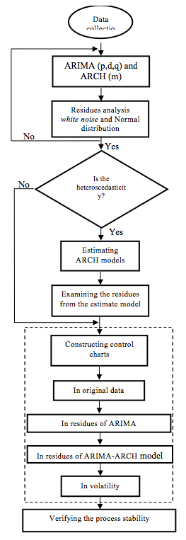
The general index number of the daily residues control is presented in percentage and refers to the period between July 2004 and May 2008 with 890 observations daily collected and to perform all steps described in the methodology the Statistica 7.0 and EViews 7.0 package will be used to perform these steps. Figure 1 shows the methodological steps in a flowchart.
Figure 1 – Methodological flowchart
The exposed method will be applied in the foundry industry where the search will be performed, it is the cast iron which, according to Chiaverini (2005), can be defined as an iron-carbon-silicon alloy, where carbon has contents higher than 2%, in excess of which is retained in solid solution in austenite, so that resulting in partially free carbon in the form of shafts or lamellae of graphite. Gray and nodular cast irons are used. The gray iron in the manufacture of materials with low mechanical resistance, such as harvesters pulleys and elevators to transport grains while the nodular iron is used in pieces such as gears of lifting loads, in particular production lines of tractors, railroads and highways.
3. Data analysis and discussion
From the use of these two types of iron characteristics arisescraps that consequently are expensive to the company. Thus, the prediction of the residues amount produced becomes extremely important for the company determining how much material is being wasted, in addition to energy, manpower and equipment being used without proper need (Frota, 1999). It is by means offorecasts that measures such as closing of contracts, inventory control and raw materials purchase can be planned and optimized.
The production of gray and nodular cast iron parts for tractors, harvesters, planters, livestock equipment and tooling are part of the production of metals studied. Parts produced are up to 80 kg in the mechanized or semi-automated process and up to 2000 kg in manual process, with installed capacity of 300 tons of pieces/month. Although the process control is made, defects such as porosity, sand erosion, high or low hardness, weld slag and cold are often generated. These defects cause some flaws such as holes and irregular gaps in the piece, rounded seams and more shiny iron when machined. There are also defects related to problems with man power and consequence in deviations in the process of forming and trimming, core shop, welding, temperature and chemical composition.
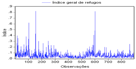
Figure 2 shows the behavior of the general index of scraps where it is observed that the series has great variability with multiple peaks, representing excess of the general index of scraps. Furthermore, there are presence of outliers, and the more distinct occurs in the observation 153 and 600 relating for the period March 2005 and February 2007, respectively.
The defects occurred in pieces are due to rechupe / porosity characterized by "holes", "empty" in the piece, both externally and internally, caused by iron temperature being too high or too low. Another factor is the chemical composition (carbon) at high levels or even a power system of the piece in the insufficient model (massalotes). Also, the entrainment of mold sand, causes holes and failures in the piece, in very irregular shapes (small / large, light / well), being caused by the use of very dry sand casting, the cast iron very fast in a mold and poor compression of the sand mold.
Figure 2 - Original series of the generalindex of scraps
The autocorrelation verification is shown by means of FAC and FACP, combined with the Ljung Box statistics that showed autocorrelation for the first 15 lags, since p-values are less than the 5% significance level.
The series stationarity is verified by means of (Phillips-Perron (PP), 1988) and (Kwiatkowski; Phillips; Schmidt; Shin (KPSS), 1992) tests. If the series is not stationary relative to average, (Pedrini; Caten, 2008) suggest using differentiations to stabilize it. In Table 1 are shown the PP and KPSS tests.
Table 1 – PP and KPSS unit root tests for the variable general index of scraps
PP |
PP |
KPSS test statistics |
KPSS |
-29.295 |
-2.864 |
0.584 |
0.463 |
*The critical value is 5%.
In Table 1, the PP test show that the null hypothesis is rejected, so the series stationary and, the KPSS test reject the null hypothesis of stationarity. Thus, the PP and KPSS tests show inclusive decision about the stationary, but according to Figure 1 we decide to adopt for the series stationarity.
Figure 1 shows that the general index of scraps are autocorrelated; therefore, one should seek a mathematical model able to eliminate the serial autocorrelation, as a way to apply control charts in the residues of mathematical model. The straight application of control charts in the original data would disagree with the assumptions necessary for the application.
Thus, one of the initial alternatives is modeling the original variable by means of linear models ARIMA (p, d q), so that modeling the conditional mean of the variable. In this case the general ARIMA model is used with parameter estimation performed through the Ordinary Least Square method. Table 2 shows competing models estimated, which have characteristics of white noise, but the chosen model is that present best AIC and BIC criteria.
Table 2 – Estimation of parameters of competing ARIMA models of
AIC and BIC criteria for the generalindex of scraps
Models |
Parameters |
AIC |
BIC |
AR(1) |
?1= 0.512 |
-2.353 |
-2.348 |
AR(2) |
?1= 0.323 ?2= 0.367 |
-2.495 |
-2.484 |
ARMA(1,1) |
?1= 0.997 θ1= -0.951 |
-2.701 |
-2691 |
IMA(1,1) |
θ1= -0.952 |
-2.702 |
-2.697 |
The best model choosen was an autoregressive with lag 1 - AR (1), the residues are investigated by mean of ACF and PACF to validate them for the application of residues control charts.
To test for the presence of heteroscedasticity in the residues of the model AR(1) is applied the ARCH-LM hypothesis test. By the hypothesis test was found: FC = 22.818 with prob = 0.000 and T.R2 = 22.296 with prob = 0.000 being F statistics and ARCH-LM significant, rejecting the null hypothesis of homocedasticity, so that the residuals of the variable general index of scraps of gray and nodular cast irons are heteroscedastic. Using the residuals of the AR (1) model, the conditional volatile is estimated using the mixed model ARIMA-ARCH in Table 3.
Table 3 - Estimation of the coefficients, standard errors, z-statistic and p-value
of the ARIMA-ARCH model for the variable general index of scraps
Method: ML – ARCH (Marquardt) – Normal Distribution |
||||||||||||
Equation for conditional mean - AR(1) |
||||||||||||
|
Coefficient |
Standard Error |
z Statistics |
p-value |
||||||||
?1 |
|
|
|
|
||||||||
Equation for conditional variance – ARCH (1) |
||||||||||||
C
|
|
|
|
|
||||||||

The estimated for mean and volatility is an AR(1)-ARCH(1) with parameters statistically significant, white noise characteristics and non autocorrelated. The parameter  of the ARCH model assumes the value of 0.222098, which shows that the conditional variance does not have a prolonged effect,after a short period of time, the series variance must converge to the historical mean. This means that the general index of scraps in the previous period does not influence strongly the next period. It also means that if the control charts show sampling points outside the limits, it should be primarily due to deviations or displacements of the mean and not due to the process variability, once the ARCH model detects little influence of variability, the effects of approximately 0.22 are too low to cause long-term effect of variability.
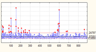
Where as when performing statistical process control the company quality center confir the achievement of data pre-control and consider the process under control. To initiate this step, we present the  control charts for individual measurements and moving range in Figures 5 and 6, using the original data set. In the
  control chart and
 were added the runs rules, which can reveal the existence of special data patterns, we can see plenty of points outside the control limits, causing high instability in the series of index of scraps of gray and nodular cast irons.
Figure 5 - |
Figure 6 - |
|
|
 chart of the general index of scraps for original data
  chartof the general index of scraps for original data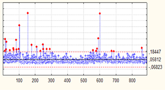

For purposes of comparison between the application of control charts in the original data set, whose variable are under autocorrelation effect, it should be noted in Figures 5 and 6. Figures 7 and 8 show the  control charts and
  applied in to the residues of AR (1) model, which are not autocorrelated.
Figure 7 - |
Figure 8 - |
|
|
 chart of residues of AR(1) model from general index of scraps
 chart of residues of AR(1) model from general index of scraps

According to the residues of the estimated model AR(1), it was drawn the  chart for individual measures and the additional criteria or sensitizing grules for Shewhart control charts Montgomery (2004) where was noticed the following situation: 9 samples in sequence are on the same side of the centerline totaling 54 sampling sites; 14 samples are in sequence alternating upwards and downwards, totaling 56 sampling points; every 3 samples drawn, 2 are located in zone A or outside it totaling 6 sample points; 15 samples in sequence situated in the zone C totaling 345 sampling points.
According to the residues of the estimated model, the moving average chart was drawn up. By implementing the runs tests were detected: 9 samples in sequence on the same side of the center line totaling 216 sampling points, 6 samples in sequence with increasing and/or decreasing trend totaling 6 sampling points; every 3 samples drawn, 2 are located in zone A or ouside it totaling 52 sampling points; every 5 samples drawn, 4 are in Zone B or ouside it totaling 80 sampling points, 8 samples in sequence located outside the zone C totaling 16 sampling points.
The control charts for residues of the mixed model AR (1)-ARCH (1) for the series general index of scraps are shown in Figure 9 and 10.
Figure 9 - |
Figure 10 - |
|
|
 chart of residues of AR(1)-ARCH(1) model from general index of scraps
 chart of residues of AR(1)-ARCH(1) model from general index of scraps
According to the residues from the estimated model, the  chart for individual measures was drawn up. By implementing the run tests were detected: 14 samples in sequence alternating upwards and downwards totaling 70 sampling points, every 3 samples drawn, 2 are located in the zone A or outside it totaling 4 sampling points; 15 samples in sequence located in the zone C totaling 330 sampling points.
According to the residues of the estimated model, the moving average chart was drawn in Figure 10 and implementing the run tests were detected: 9 samples in sequence on the same side of the centerline totaling 243 sampling points, 6 samples in sequence with increasing and/or decreasing trend totaling 6 sample points;every 3 samples drawn 2 are located in the zone A or outside it totaling 46 sampling points, every 5 samples drawn, 4 are in Zone B or outside it totaling 76 sampling points.
It should be noted that modeling AR (1)-ARCH(1), where only the second model part is responsible for determining the volatility intrinsic to the data. According to the estimated values for volatility of the estimated model and its behavior can be seen at Figure 11.
Figure 11 - Conditional volatility of the mixed model AR (1)-ARCH (1)

Analyzing Figure 11, which represents the conditional volatility, the mixed mathematical model AR (1), ARCH (1), captured periods of greater variability, represented by clusters of volatility, which was also reflected in the residue model which was used to plot the control. Noting Figures 5-10, it is apparent that the points detected out of control are close to or surrounding the values when there were volatility peaks shown in Figure 11, in observations 15, 17, 18, 23, 45, 67, 84, 85, 99, 104, 179, 180, 235, 251, 293, 294, 585, 593, 594, 603, 604. Thus, it can be said that a detailed analysis of the intrinsic data volatility must be conducted so that the interpretation of control charts to become more effective.
Regarding the results obtained after the application of control charts  , the following considerations on the general index of scraps are made:
When analyzed the original data of the variable under study, there were 307 sampling points outside the control limits. While analyzing the residues from the AR (1) model, there was 461 sampling points outside the control limits. Going beyond the research, using the residuals from the mixed model AR (1)-ARCH (1), there was 404 sampling points outside the control limits. Thus it is clear that the autocorrelation actually influences the detection of sampling points out of control and that the best the model is estimated, the best and more accurate are the residues, bringing improment to the performance of control charts.
Regarding the results obtained after application of  control charts, the following considerations for the general index of scraps are shown: When analyzing the original variable, there was 299 sampling points outside of control limits, but when the chart was applied to the residues of the AR (1) model there was 370 sampling points outside the control limits and in this case the dataset is already free of autocorrelation. Where as when the mixed model AR (1)-ARCH (1) is estimated and the residues are used, there are 371 sample points outside the control limits, in this case we have reliable residues, since the modeling is more robust, taking into consideration the implicity variability to the observations.
The claims mentioned above show that, after fitting the data using the mixed model, only the autocorrelation effect has been eliminated, but it is necessary to quantify the volatility influence on the process that in this case was low at around 0.22. Thus, it is justified the accuracy of the mixed model, which showed a significant improvement in detecting sampling points outside the control limits in comparison with the AR (1) model, whose have the parameter AR with different values when the mixed estimation is considered, first the parameter was ?1= 0.512 and changed to ?1 = 0.772429.
4. Conclusions and final remarks
The methodology, using residues control charts for autocorrelated processes, showed an alternative way to evaluate the process and treat the existing data dependency, whose can be thought in mean dependency treted using ARIMA models and, the second one is the volatility, that is treated using ARCH models, these two kinds of measurements are the first and second moments used to characterize a variable.
The AR-ARCH modeling provided analyzing the mean process characterizing it for stability and in addition to this analysis, it is verified the volatility behavior, where the persistence reveled by the parameter of ARCH model will not affect the process for a long time. Thus, it is possible to verify that a volatility parameter below 0.6 shows that the fluctuations will not persist affecting future production, another interpretation is that the volatility below 0.6 the variability may be inherent to the process and possibly do not affect the control limits reflecting just a common cause is acting.
Finally, the AR-ARCH model was crucial in the application of control charts, once it enabled that the autocorrelation present in the data were incorporated into the forecasting model providing residues with more reliability to assess the stability of scraps production in the production process, since using the original data would not be possible to obtain a correct interpretation due to serial dependence. The process can be classified as unstable showing several sampling points outside the control limits.
It is suggested as a future study using other mathematical models and the application of other control charts as a way to spread the application of ARCH models in industry.
5. Acknowledgements
Indústria de Fundição Metalúrgica Candeia Ltda for data provided, the CNPq and CAPES for partial financial support for research development. The third author thanks CAPES Process BEX 1784/09-9 - CAPES. We thank the anonymous reviewers for the critical evaluation and improvement provided to this article.
6. References
Alwan, L. C.; Roberts, H. V. (1988); "Times series modeling for statistical process control"; Journal of Business & Economics Statistics; v. 6; n. 1; 87-95 p.
Acquah, H. G. (2010); "Comparison of Akaike information criterion (AIC) and Bayesian information criterion (BIC) in selection of an asymmetric price relationship"; Journal of Development and Agricultural Economics; v. 2 (1); 001-006 p.; january.
Akaike, H. (1973); Information Theory and an Extension of the Maximum Likelihood Principle; In: B.N. Petrov and F. Csaki (eds.); 2nd International Symposium on Information Theory: 267-81; Budapest: Akademiai Kiado.
Baillie, R.; Chung, C. F.; Tieslau, M. A. (1996); "Analyzing inflation by the fractionally integrated ARFIMA-GARCH model"; Journal of Applied Econometrics; v.11; 23-40 p.
Bollerslev, T. (1986); "A conditional heteroskedastic time series model for speculative prices and rates of return"; Journal of Econometrics; v. 69; 542-547 p.
Box, G. E. P.; Jenkins, G. M. (1970); Time series analysis: forecasting and control. San Francisco: Holden-Day.
Box, G. E. P.; Jenkins, G. (1976); Time series analysis: forecasting and control. San Francisco: Holden-Day.
Box, G. E. P.; Jenkins, G. M.; Reinsel, G. C. (1994); Time series analysis: forecasting and control; 3. ed.; San Francisco: Holden-Day.
Campos, K. C. (2007); "Análise da volatilidade de preços de produtos agropecuários no Brasil"; Revista de Economia de Agronegócio; v. 5; n. 3; 303-328 p.
Chiaverini, V. (2005); Aços e ferros fundidos; São Paulo; ABM.
Ehlers, R. S. (2009). Análise de séries temporais; In: Notas de aula de séries temporais; São Paulo: USP;. Disponível em: <http://www.icmc.usp.br/~ehlers/notas/stemp.pdf>; Acesso em: 13 dez. 2010.
Engle, R. (1982); "Autoregressive conditional heteroscedasticity with estimates of the variance of United Kingdom inflation"; Econométrica; Chicago; v. 55; n. 4; 987-1007 p.; july.
Frota, A. (1999); O barato sai caro! Como reduzir custos através da qualidade?; Rio de Janeiro: Qualitymark Editora.
Gujarati, D. N. (2006); Econometria Básica; 3.ed.; São Paulo: Makron Books.
Harris, T.J.; Ross, W. H. (1991); "Statistical process control procedures for correlated observations";The Canadian Journal of Chemical Engineering; v. 69; 48-57 p.
Huang, X.; Liu, W. (2009); "Properties of some statistics for AR-ARCH model with application to technical analysis"; Journal of Computational and Applied Mathematics; v. 225; 522-530 p.
Khashei, M.; Bijari, M. (2011); A novel hybridization of artificial neural networks and ARIMA models for time series forecasting; Applied Soft Computing; v. 11; 2664-2675 p.
Kwiatkowski, D.; Phillips, P. C. B.; Schmidt, P.; Shin, Y. (1992); "Testing the null hypothesis of stationarity against the alternative of a unit root"; Journal of Econometrics; v. 54; 159-178 p.
Lee, C.-M; Ko, C.-N. (2011); Short-term load forecasting using lifting scheme and ARIMA models; Expert Systems with Applications; v. 38; 590-591 p.
Lamounier, M. W. (2006); "Análise da volatilidade dos preços no mercado spot de cafés do Brasil"; Organizações Rurais & Agroindustriais; v. 8; n. 2; 160-175 p.
Marchezan, A.; Souza, A. M. (2010); "Previsão do preço dos principais grãos produzidos no Rio Grande do Sul"; Ciência Rural; Santa Maria; v. 40; n. 11; 2368-2374 p.; november.
Montgomery, D. C. (1997); Introduction to statistical quality control; 3.ed.; New York: John Wiley & Sons, Inc.
Morettin, P. A.; Toloi, C. M. C. (2004); Análise de séries temporais; 2. ed.; São Paulo: Edgard Blücher.
Morettin, P. A.; Toloi, C. M. C. (2008); Econometria financeira: um curso em séries temporais financeiras; São Paulo: Blücher.
Pedrini, D. C.; Caten, C. S. (2008); "Comparação entre gráficos decontrole para resíduos de modelos"; GEPROS; Gestão da Produção, Operação e Sistemas; v. 3; n. 4; 123-140 p.; out-dez.
Pedrini, D. C.; Caten, C. S. (2011); "Método para aplicação de gráficos de controle de regressão no monitoramento de processos"; Produção; v. 21; n. 1; 106-117 p.
Perron, P. (1988); "Trends and random walks in macroeconomic time series"; Journal of Economic Dynamics and Control; v. 12; 297-332 p.
Schwarz, G. (1978); Estimating the Dimension of a Model. Annals of Statistics 6: 461-464.
Stock, J. H.; Watson, M. W. (2004); Econometric; São Paulo: Addison Wesley; 485 p.
Silva, W. S.; Sáfadi, T.; Castro Jr., L. G. (2005); "Uma análise empírica da volatilidade do retorno de commodities agrícolas utilizando modelos ARCH: os casos do café e da soja"; Revista de Economia e Sociologia Rural (online); v. 43; n. 1; 119-134 p.; jan-mar.
Souza, A. M.; Souza, F. M.; Ferreira, N.; Menezes, R. (2011); "Eletrical energy supply for Rio Grande do Sul, Brazil, using forecast combination of weighted eigenvalues"; GEPROS: Gestão da Produção, Operações e Sistemas; ano 6; n. 3; 23-39 p.; jul-set.
Tsai, T.; Chiang, Y.; Wu, S. (2004); Conditional maximum likelihood estimation for control charts in the presence of correlation; Brazilian Journal of Probability and Statistics; v. 18; n. 2; 151-162 p.; december.
Wasserman, L. (2000); Bayesian Model Selection and Model Averaging; J. Math; Psychol; v. 44; 92-107 p.
Zhu, F.; Wang, D. (2010); Diagnostic checking integer-valued ARCH (p) models using conditional residual autocorrelations; Computational Statistics and Data Analysis; v. 54; p. 496-508 p.