ISSN 0798 1015

Vol. 38 (Nº 57) Year 2017. Page 3

Generation of Forecasts Based on the Analysis of the Real Behavior of the Demand of a Colombian Textile Company

Generación de pronósticos basados en el análisis del comportamiento real de la demanda de una empresa textil colombiana

Ricardo PRADA O. 1; Pablo C. OCAMPO 2

Received: 14/07/2017 • Approved: 10/08/2017

Content

1. Introduction

2. Theoretical framework

3. Methodology of the investigation

4. Results of the application of the forecast models to the historical data of demand of the product line

5. Statistical models of prognosis for the short term

6. Conclusions

References

1. Introduction

Building a supply chain in an advantageous position in Latin America implies overcoming several obstacles typical of the region, such as long distances between major cities and inefficient road transport infrastructure, which is the most used medium. Land transport in the region is slow traffic, with an average speed of 6 to 50 mph and high risk due to unsafe conditions. In this concept, Colombia has an index of use of 77%.

According to the Textile and Clothing Business Plan of the Productive Transformation Program (PTP); The consumers of the three continents look for a better quality at a lower price, combining low-cost garments with high-end garments, thereby increasing the level of importance of corporate social responsibility. As for the product offered, it tends to establish economic prices in the three continents. The quality of the proposed product is increased by assembling more number of collections per year. As far as marketing is concerned, there is a tendency to reduce the actors in the different channels: department stores, discount stores, national chains and specialized stores. The internet begins to be relevant as a sales channel, representing a 25% development for the Latin American region and with a tendency towards a full identification of suppliers and marketers. Finally, in terms of supply, the Latin American region must make more progress in the development of logistical management tools to optimize the response to large companies that subcontract their production; In addition to reducing the number of suppliers usually handled (Ministry of Commerce, Industry and Tourism, 2009, pp. 104-108).

The clothing and textiles sector in Colombia is concentrated primarily in Bogotá and Antioquia, with a combined share of 77.44% over the national total. Within this sector different actors are identified that form a productive chain structure of 5 links: the first one is the suppliers of fibers, spinning and chemical products for textile use; The second, producers of textiles and supplies such as foams, zippers and buttons; The third, companies engaged in the manufacture of clothing and household; The fourth, the merchants of textiles, garments and fibers wholesale and retail; And finally, local, national and international consumers. SMEs represent 80.8% of the total (Superintendency of Corporations, 2013). 

On the other hand, the present state of the application of management methods in the production chain of the textile sector in Colombia, has an approximate level of 95% of advance in supply management and 70% in the demand managment. Likewise, 25% of companies in the sector have their own transport equipment, 33% have their own warehouse and 30% have warehouses for leasing, while 79% use spreadsheets for management, 34% Uses electronic data interchange and 25% has electronic catalogs (Zuluaga & López, 2010).

According to Zuluaga & López (2010), the forecasting methods for SMEs are mostly qualitative and powerful when suppliers and large clients are involved in this work, who have first-hand information on market behavior; However, according to the same study cited, there is a low penetration of ICT in SMEs, which makes it financially unfeasible to establish collaborative trade schemes between suppliers and customers. 

According to the economic and business profile of the western industrial zone in Bogotá (Bogota Chamber of Commerce, 2007, page  52), there are 1487 companies belonging to the Textile - Clothing sector,  which have the potential to be linked to a production chain, of which 42 are suppliers of inputs, 780 are engaged in processing and 665 are engaged in marketing. In the transformation link, to which the Colombian textile company belongs, there are 780 companies that are mostly engaged in the manufacture of garments, household and outdoor clothing; Of these companies 719 are engaged in clothing; And in turn this group, 10.99% are classified as small companies, as the Colombian textile company. On the other hand, in the marketing link are 665 companies that are mostly engaged in the retail sale of finished products such as fabrics, cloths, clothing, industrial clothing and sportswear; Of these, 79.25% are engaged in the retail trade of finished products, the Colombian textile company belonging to this group.

The demand-driven supply chain concept has gained relevance (Cooke, 2013). This approach refers to the impact of the interpretation of the demand behavior along the links from the final consumer to the initial suppliers, with a "whiplash" effect as information is disseminated to the first suppliers ( Lipton, 2013). The effect results in excess or depleted inventory, since each link typically makes its demand forecasts according to its specific client, that is, the next link in the chain; In this way, the actor located in the link in contact with the final consumer is the one who can generate forecasts of greater precision, due to the access that has to the actual data of requirements. 

The present research aims to generate forecasts based on the analysis of the real behavior of the demand. The assertive reading of the demand results, through the application of strategies of promotion, prices and development of new products, facilitates their modification, offering a profitable response according to the strategic planning of the company and driven towards the first links of the chain of supply. This alignment allows reducing the number of depleted and becomes important for the e-commerce sales channel, where the consumer can change brands with ease. Greater sensitivity to real consumer demand is achieved (Cedol, 2013).         

2. Theoretical framework

According to Chase (2011) there is a first classification of demand forecasts, defining them in Strategic, which are the basis for decision makingin terms of capacity, process design, procurement, location, distribution, sales planning and operations; Secondly, in the medium and long term, that is, a term of 3 months to more than 2 years; And finally, in Tactics, which are the basis for short-term decision making, ie weeks and up to 3 months, in terms of production planning, operator scheduling, and restoration of security inventory levels. 

A second level of classification of the forecast, typifies Hanke (2010, p. 3) in Qualitative, which is obtained through the "personal judgment of the forecaster" as a product of a mental manipulation of historical data, not including formal mathematical analysis of these; And Quantitative,Which is the result of statistical analysis of time series, ie historical sales data, to obtain a prediction of future demand. Other authors (Chase, 2011, p. 485) (Hanke, 2010, p. 3), y (James, 2012, p. 81)  suggest that a joint forecast be developed between the two techniques, tools of statistical analysis together with the judgment of the expert, to obtain an approximate prognosis to the reality, bearing in mind that it is not possible to obtain a perfect prognosis and errors of accuracy are inevitable.Thus, when making a quantitative analysis of the series of data that correspond to the historical data of sale of the underwear line, the following basic components of the time series must be taken into account:

• Stationary Patterns:  Corresponds to the arithmetic mean of the data over a period of time, and applies to those series that vary around a fixed level over time (Hanke, 2010, p.  15, 72).

• Trend Patterns: They represent the growth or decline of the series that persists over time. It is the starting point for developing a forecast because the trend line allows identifying the behavior of the data, then choose the mathematical model that best fits; At this point it's combined the forecast tool used (excel spreadsheets, software like WinQSB, and in general, statistical packages) along with the judgment of the forecaster, since it is the direct observation of the trend line presented by the data , which allows to choose a specific mathematical model (Linear, S curve, Logarithmic and exponential) (Saint-Jacques, 2008) (Chase, 2011, p.  487) (James, 2012, pp.  82-83) (Hanke, 2010, p.  63 y 78).

• Seasonal Patterns: They represent the fluctuations that take place in the course of a year and are repeated annually. Example: demand for specific items during winter and summer (Chase, 2011, p.  492) (James, 2012, p.  84) (Hanke, 2010, p.  64).

• Cyclic Patterns: These are patterns of oscillation that are related to the tendency of the data in the long run, with no fixed periods. The cyclical pattern is the result of changes in general economic conditions and the way they affect the particular industry or sector; Thereby, are unstable because the affectation to each unit of the sector depends on their individual reaction (Chase, 2011, p.  492) (James, 2012, p.  83) (Hanke, 2010, p.  63).

• Random Variation: These are random variations, caused by unforeseen events, not explained by trend, cyclical or seasonal patterns (Chase, 2011, p.  486) (James, 2012, p.  84).

• Autocorrelation:  Indicates that the expected value at any given time has a high correlation with its own previous observations, and shows that the data are not random (Chase, 2011, p.  486) (Hanke, 2010, p.  69).

The choice of the statistical model to be used to obtain the forecast is developed according to the patterns presented in the time series. In that way, Chase (2011) recommends as a good practice, to test with more than one model and to determine which gives the lowest margin of error, which corresponds to the difference between the actual value and the predicted value for the same period of time; And a periodic review of the fit of the chosen model should be made.

The results should be compared with the data collected previously, to determine the degree of fit between the historical and analytical findings. The comparison should focus on identifying significant differences and determining possible sources of errors. Potential errors may result from inaccurate or incorrect data entry, inadequate or inaccurate analysis procedures, or validation of non-representative data (Bowersox et al., (2007) p.  333).

Several methods for forecasting use statistical criteria and relation, standard deviation, correlation coefficient are applied. These guidelines allow the measurement model to have higher quality. A necessary condition for the review is that the residue is composed only of random characteristics such as self-correlation of residues. In addition, if the trend, seasonality or cycle characteristics appear in the residuals, the models will be improved by any other method use or parameter modification (Jaffeux, 2002, p.  375). The ability to see the future would be priceless, but the most you can do is predict and list all possible solutions and the likelihood of a result. Filling the constant needs of customers, would be extremely easy in logistics; The problem is that customer demands are changing, generating excess inventory, incomplete orders or last minute deliveries (Long, 2011).

According to Hanke (2010, p. 82) there are several metrics for the margin of error that allow, on one hand, to know the behavior of errors during the time horizon analyzed; And on the other, to define the forecast model for better fit to the data, according to the lowest margin of error acquired. Thus, the following metrics are defined as measurement indicators for the forecasts:

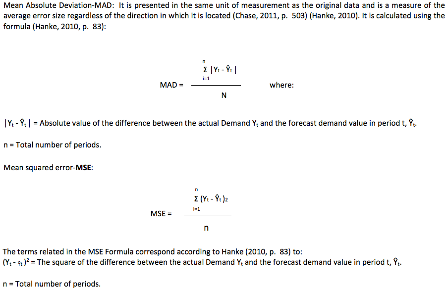
This measurement "penalizes" the errors of large margin by being squared, which allows to identify the model of forecast that casts small errors but that eventually gets to produce errors of great measure. Its unit of measure is equal to that of the original data.

According to David (2010, pp.  68-70), the most important factors for a successful supplier-buyer relationship are related to the supplier's responsiveness to meet the ordered requirements and clear product specifications. In practice, three types of relationship between suppliers and customers are identified:  Transactional, which is the basic type, corresponding to the independent exchange of goods or services and money; Collaborative, which refers to shared efforts and planning,  interdependence, and effective communication, and Strategic Alliance, in which institutional trust is developed and the parties share strategic information regarding their interdependent operations.

3. Methodology of the investigation  

The applied research approach is a quantitative one, characterized by following a sequential order, starting from an idea that is intentionally delimited until it becomes concrete, and then consult the pertinent literature, corresponding to previous studies of the subject and theories that will guide the study , In order to build a theoretical framework (Hernández, Collado, & Baptista, 2010). It is also descriptive, as it seeks to study the characteristics of the behavior of the demand for the underwear line of the Colombian textile company. 

Historical data of monthly demand for the underwear line were collected, corresponding to the period from January 2013 to September 2016. Primary information pertinent to the study was collected, corresponding to the monthly historical data of sales of the underwear line of the Colombian textile company for the period 2013 - 2016. A physical analysis of the sales invoices of the company corresponding to the period analyzed was performed, discriminating sales of the line. 

To determine the sample size, at least 4 years of historical behavior is included; In this way the margin of error that can be presented is reduced to the maximum possible. We considered a sample size n = 45 data, corresponding to the monthly sales of the line for the mentioned period. 

Short, medium and long term forecast models were applied for the historical demand data of the underwear line, determining the error associated with the calculations and choosing the model that yields the least margin of error.  In the execution of this activity will take into account the theoretical position addressed. Chart 1 provides the parameters for the calculation of forecasts for this research.

Chart 1:  Forecast Models to be applied and Software Used

Source:  Author

4. Results of the application of the forecast models to the historical data of demand of the product line

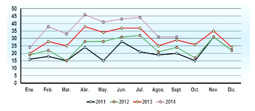
The underwear line of the Colombian textile company, consists of four products that aggregate the following historical behavior of Demand for the period 2013 - 2016

Figure 1
Historical Behavior of Demand in units of the underwear line 2013 - 2016. 

Source: Prepared by the author based on
analysis of data collected in the company.

As shown in figure 1, the demand for the product line has been increasing month-on-month for the period 2013 - 2016, presenting similar behavior of low demand peaks for the months January, March, May, August, October and December; And of greater demand in the months of February, April, June, July, September and November. Chart 2 presents the monthly data series collected, with which Figure 1 was elaborated.

Chart 2
Time series in units 2013 - 2016.

Source:   Prepared by the author based on
analysis of data collected in the company.

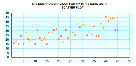
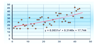
To identify cyclical patterns in the data, the total demand behavior must be analyzed. Figure 2 presents the 45 historical data collected in a scatter plot.

Figure 2
Behavior of Demand for n = 45

Source: Prepared by the author based on
analysis of data collected in the company.

5. Statistical models of prognosis for the short term

As it was approached in the theoretical position, statistical models of forecasting were applied for the short term, which are developed below.

5.1. Moving Averages

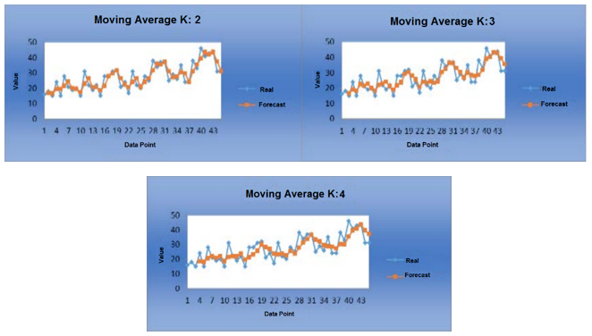
As mentioned in the theoretical position, there must be a minimum of 4 to 20 data for the application of this model. As the size of the sample n = 45 is adjusted to this restriction and the model can be applied, taking into account that if there is seasonal component a group of data of the same behavior must be taken for the calculation of the moving average. Thus, taking into account groups of size k = 2, 3 and 4 data to calculate the moving average, the following forecast graphs are obtained:

Figure 3
Forecasts obtained with Moving Averages K = 2, 3, 4 Data.

Source: Prepared by the author based on
analysis of data collected in the company.

As can be seen in Figure 3, the forecast obtained with Moving Media corresponding to k = 2, is the one that best adjusts to the behavior of the data. This will be evidenced by the calculation of the margin of error indicators. When calculating the forecast for periods 46 to 48, and also the error indicators, the following data are obtained:

Chart 3
I predict to 3 months applying moving averages
k = 2, 3 and 4. Calculation of Error Indicators.

Source: Prepared by the author based on analysis
of data collected in the company.

As shown in Chart 3, the error measurement indicators yield favorable results for the moving average with k = 2.

5.2. Exponential Smoothing.

As approached in the theoretical position, to apply this model must have a minimum of 3 data; So the sample size n = 45 is adjusted to this restriction and the model can be applied. Thus, taking into account different values ​​of the constant α (option 1 α = 0.1, option 2 α = 0.2, option 3 α = 0.3 and option 4 α = 0.6) to perform prediction calculations, the following forecast graphs are obtained:

Figure 4
Forecasts obtained with α = 0.1, 0.2, 0.3 and 0.6 for the Exponential Smoothing Model.

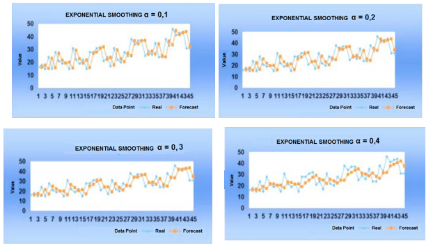
Source: Prepared by the author based on
analysis of data collected in the company.

As can be seen in Figure 4, the forecast obtained with Exponential Smoothing corresponding to a α= 0.1 is the one that best adjusts to the behavior of the data. This will be evidenced by the respective margin of error metrics. On the other hand, when calculating the forecast for periods 46 to 48 and the mentioned metrics, the following data are obtained:

Chart 4
3-month forecast applying α = 0.1, α = 0.2, α = 0.3 and
α = 0.6 for the Exponential Smoothing Model. Calculation of the Error.

Source: Prepared by the author based on
analysis of data collected in the company.

As can be seen from Chart 4, the error measurement indicators show favorable results for the exponential smoothing corresponding to α = 1, presenting higher and higher results as the α value increases. Thus, within the forecasts calculated with the exponential smoothing model, the one corresponding to α = 0.1 is the one with the best performance.

5.3. Holt Linear Exponential Smoothing

As approached in the theoretical position, to apply this model must have a minimum of 3 data; So the sample size n = 45 is adjusted to this restriction and the model can be applied. We defined different values ​​for the α and β constants (option 1: α = 0.1 and β = 0.1, option 2 α = 0.2 and β = 0.2, option 3 α = 0.3 and β = 0.3, option 4 α = 0.3 and β = 0.7 ), In order to perform the prediction calculations, obtaining the following forecast graphs in the Win QSB program (Option: Forecasting:  Single Exponential Smoothing with Trend):

Figure 5
Forecasts obtained with 4 options of α and β for the Holt Linear Exponential Smoothing Model

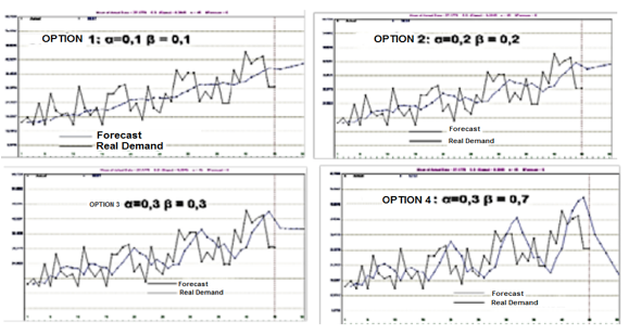
Source: Prepared by the author based on analysis
of data collected in the company.

It is observed in figure 5, that the forecast corresponding to α = 0.3 and β = 0.7 is the one that best adjusts to the behavior of the data. However, this first analysis must be contrasted with the respective margin of error metrics.  On the other hand, when calculating the forecast for periods 46 to 48 and the mentioned metrics (According to the option Forecasting:  Single Exponential Smoothing with Trend, WinQSB program), the following data are obtained:

Chart 5
3-month forecast applying Holt Linear Exponential
Smoothing Model. Calculation of the Error.

Source: Prepared by the author based on
analysis of data collected in the company.

As can be seen from Chart 5, the error measurement indicators show favorable results for the prognosis obtained with the exponential smoothing corresponding to α = 1, β = 0.1; presenting higher and higher results as the values of α and β are increased. Thus, within the forecasts calculated with the holt lineal exponential smoothing model, the one corresponding to α = 0.1 and β = 0.1 is the one with the best performance.

5.4. Winters Multiplicative Seasonal Exponential Smoothing

As addressed in the theoretical position, to apply this model must have a minimum of 2 data per Station; So the sample size n = 45 is adjusted to this restriction and the model can be applied. The values ​​of α, β, and γ are defined as option 1: α = 0.1, β = 0.1, and γ = 0.1, option 2: α = 0.2, β = 0.2, and γ = 0.2, option 3: α = 0.3 , Β = 0.3, and γ = 0.3 and option 4:  α = 0.4, β = 0.4, and γ = 0.4, in order to perform the prediction calculations, obtaining the following forecast graphs in the Win QSB program (Option:  Forecasting, Holt-Winters Multiplicative Algorithm)

Figure 6
Forecasts obtained with 4 options of α and β for
the Winters Multiplicative Seasonal Exponential Smoothing Model

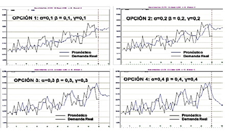
Source: Prepared by the author based on
analysis of data collected in the company.

Figure 6 shows that the forecast corresponding to α = 0.4, β = 0.4 and γ = 0.4 appears to be the most accurate to the behavior of the data. However, this first analysis must be contrasted with the respective margin of error metrics.  On the other hand, when calculating the forecast for periods 46 to 48 and the mentioned metrics (According to the option Forecasting:  Holt-Winters multiplicative algorithm, WinQSB program), the following data are obtained:

Chart 6
3-month forecast applying Holt Linear Exponential
Smoothing Model. Calculation of Error Indicators.

Source: Prepared by the author based on
analysis of data collected in the company.

As can be seen from Chart 6, the error measurement indicators show favorable results for the prognosis obtained with the exponential smoothing corresponding to α = 1, β = 0.1; presenting higher and higher results as the values of α and β are increased. Thus, within the forecasts calculated with the Winters Multiplicative Seasonal Exponential Smoothing Model, the one corresponding to α = 0.1, β = 0.1 and γ=0.1  is the one with the best performance.

Statistical models of forecasting were also applied for the medium term, the first one being Linear Regression. As addressed in the theoretical position, to apply this model must have a minimum of 10 to 20 data; So the sample size n = 45 is adjusted to this restriction and the model can be applied. First, the correlation coefficient of the data is determined, which is a measure of the degree to which two variables are linearly related to each other; Can have values ​​between 1 and 1, which are interpreted taking into account that if r = 1 the data are perfectly linearly related to a positive trend; And yes r = -1 the data are perfectly linearly related to a negative trend (Hanke, 2010, p.  37). 

For the data of the analyzed sample n = 45, the correlation coefficient presents a value of 0.7188, obtained in Excel spreadsheet, through the option Data analysis:  Regression. This value indicates that the data have high positive linear correlation, because its value is close to 1. 

Figure 7
Linear regression

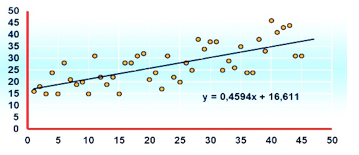
Source: Prepared by the author based on
analysis of data collected in the company.

Using the Excel spreadsheet for trend data, y = 0.4594x + 16.611, you can make forecasts for the following periods, which correspond to 6, according to the methodological design, as follows:

Chart 7
Prognosis at 6 months applying Linear Regression. Calculation of Error Indicators.

Source: Prepared by the author based on
analysis of data collected in the company.

As shown in Chart 7, the error measurement indicators show favorable results that must be contrasted with the other statistical forecast models applied in order to choose the best performance model, that is, the one that yields metrics with more values low.

5.5. Classic Decomposition                

As approached in the theoretical position, to apply this model must have a minimum of 5 data per Station ; So the sample size n = 45 is adjusted to this restriction and the model can be applied. Given that for the last year of analysis there are 9 data (corresponding to the monthly sales from January 2013 to September 2016, as shown in Chart No. 2), it is established to define the Station with 9 periods Monthly; In order to obtain a prognosis at 6 months, equivalent to future periods 46 - 51. Thus, it starts by grouping the 45 available data into groups of 9 data in order to make moving averages, as seen in Chart 8: 

 Chart 8
Step 1 - Model of Forecast Classic
Decomposition: moving average

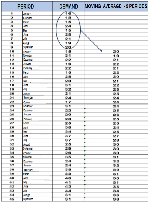
Source: Prepared by the author based on
analysis of data collected in the company.

After performing the calculations of the moving average, we proceed to calculate the seasonality factor, as seen in Chart 9.

Chart 9
Step 2 - Model of Forecast Classic Decomposition:  Seasonality factor.

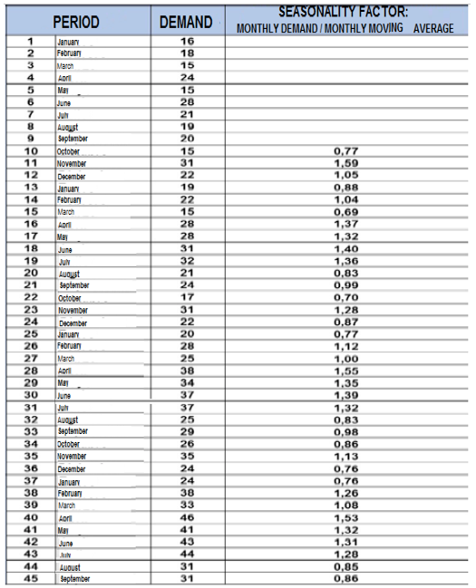
Source:   Prepared by the author based on
analysis of data collected in the company.

Then the average seasonal index for each month is calculated, based on the seasonal factors previously obtained and that can be observed in Chart 10.

Chart 10
Step 3 - Model of Forecast Classic Decomposition:
 Monthly Average Seasonality Factor.

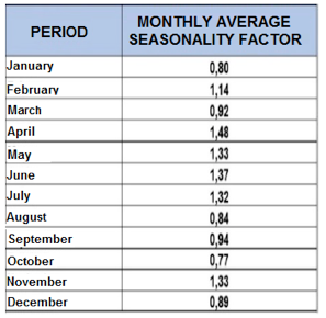
Source: Prepared by the author based on
analysis of data collected in the company.

With the data of the monthly average seasonality factor mentioned in Chart 10, we proceed to calculate the adjusted Seasonality Factor for each month, as seen in Chart 11:

Chart 11. Step 4 - Model of Forecast Classic Decomposition:
Monthly Adjusted Seasonality Factor.

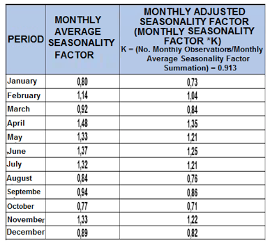
Source:   Prepared by the author based on analysis of data collected in the company.

The next step corresponds to the calculation of the cyclic Factor, as seen in Chart 12

Chart 12
Step 5 - Model of Forecast Classic
Decomposition:  Cyclic Factor.

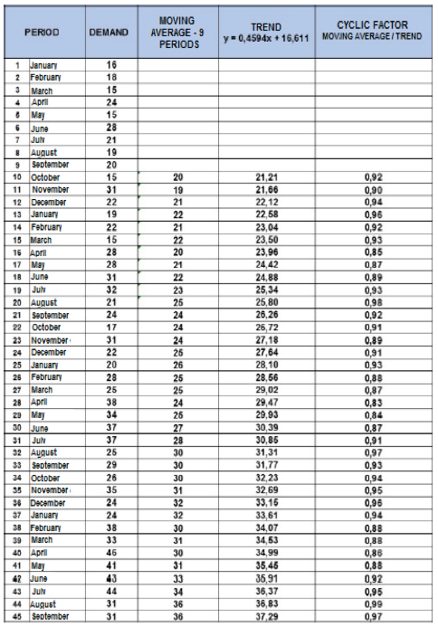
Source: Prepared by the author based on analysis of data collected in the company.

Then the average cyclical index for each month is then calculated, based on the cyclical factors previously obtained and which can be observed in Chart 12.

Chart 13
Step 6 - Model of Forecast Classic
Decomposition:  Monthly Cyclic Factor.

Source: Prepared by the author based on
analysis of data collected in the company.

Finally, the prognosis is calculated as shown in Table 14, using the formula Yt = St * Tt * Et; Taking into account that Y is the value of the forecast, St is the trend value for each period according to the linear regression calculation for the data and that corresponds to a = 0.4594x + 16.611; Tt is the cyclic factor for each month; And finally Et is the monthly Seasonal Factor adjusted for each month and calculated as shown in Chart 11.

Chart 14
6-month forecast applying Classical Decomposition. Calculation of Error Indicators.

Source:   Prepared by the author based on
analysis of data collected in the company.

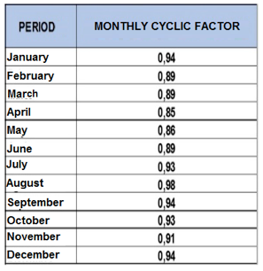
As shown in Chart 14, the error measurement indicators show favorable results that should be compared with the other statistical models of medium and long-term forecasting in order to choose the best fit. Statistical models of forecasting were applied for the long term, the first one being the Exponential Trend. As approached in the theoretical position, to apply this model must have a minimum of 10 data; So the sample size n = 45 is adjusted to this restriction and the model can be applied. It starts by applying the exponential curve to the scatter plot of the data, according to the option add trend line of the Excel spreadsheet, obtaining the exponential equation adjusted to the data, as can be seen in the graph: 

Figure 8. Exponential Trend

With the formula obtained by means of the spreadsheet Excel for the trend of the data, y = 17,416e0.0173x, the forecasts can be made for the following periods, like this: 

Chart 15
Forecast to 12 months applying Exponential
Trend. Calculation of Error Indicators.

Source:  Prepared by the author based on
analysis of data collected in the company.

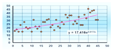
As shown in Chart 15, the error measurement indicators show favorable results that should be compared with the other statistical models of long-term forecasting. In order to apply the Quadratic Tendency model as described in the theoretical position, a minimum of 10 data must be available; So the sample size n = 45 is adjusted to this restriction and the model can be applied. The Quadratic Trend curve was applied to the scatter plot of the data, according to the option add trend line of the excel spreadsheet:  Polynomial order 2, obtaining the quadratic equation adjusted to the data.

Figure 9. Quadratic Trend.

With the Excel spreadsheet for the trend of the data, y = 0.0031x² + 0.3148x + 17.744, the forecasts can be made for the following periods as well: 

Chart 16
Forecast to 12 months applying Quadratic
Trend. Calculation of Error Indicators.

Source: repared by the author based on analysis of data collected in the company.

As shown in Chart 16, the error measurement indicators show favorable results that should be compared with the other statistical models of long-term forecasting. 

It is good practice to apply to the historical Demand data several Forecast models, choosing the one that best fits the behavior of the data. In order to offer the proposed forecast model for the product line,This choice is made according to the model that gives the lowest margin of error, which for the case of this study contemplates three indicators:  MAD, MSE and MAPE. 

Chart 18 presents a summary of each of the methods applied with the results obtained for these indicators, taking into account that in the cases of forecast models corresponding to Moving Averages, Exponential Smoothing, Holt Linear Exponential Smoothing and Winters Multiplicative Seasonal Exponential Smoothing. A pre-selection was made according to the options previously defined in the methodological design to apply the forecast, choosing in each of the models the option that presented better performance.  

Chart 17
Summary Margin error indicators for each model of Forecast applied to the demand of the underwear line

Source: Prepared by the author based on
analysis of data collected in the company.

As can be seen in Table 17, for the behavior of the demand for the medium-term underwear line, it is convenient to use the classical decomposition model, since it yields an indicator of better performance than linear regression. With respect to the short-term forecast models, the demand behavior is adjusted with a smaller margin of error to the exponential smoothing model for α values ​​close to zero. Lastly, when analyzing the results of error indicators for long-term models, the indicators show very similar values, but the Exponential Trend model is chosen because of the three indicators analyzed, it shows a better performance in two respects To the Quadratic Trend model. 

According to the quantitative analysis of the forecast models applied, they would be chosen as viable forecasting methods to predict the future demand of the underwear line:  Exponential Smoothing with α values ​​close to zero for the short term; In the medium term the Classic Decomposition and Exponential Trend for the long-term. The decision on the model to be applied must be complemented with the subjective criterion of the one who makes the calculations, which is usually the management.

6. Conclusions

From the results it is evident that it is possible to articulate projects of a collaborative type in the supply chain of the underwear line; Involving the actors Colombian textile company and level 1 suppliers; Starting with the administration of demand and supply management, taking as a starting point the calculation of demand forecasts for the line for the short, medium and long term; And in turn, share this information to the first links of the chain, in order to improve the visibility of the first links, and jointly improve the performance of the entire chain in terms of decreasing excesses and no available inventory.

It was evidenced the importance of the different collaborative models in the company, involving suppliers and the internal part of the company, where, through the implementation of forecast models, costs, response time and standardization of operations were improved, and service levels increased. Within the company's operations, the supply chain management strategy must be strengthened to improve collaboration among the many players in the company's value network.

The process of sharing strategic information such as demand forecasts implies the implementation of technological platforms that allow the exchange and generation of data in real time, such as ERP software adapted for companies such as SMEs, such as the colombian textile company. Therefore, implementing this type of software represents an investment of high profitability because it avoids duplication of activities, optimizes response times, represents a saving due to the rational use of paper and conducive to the correct flow of information, capital,  goods and services along the chain or network to which SMEs belong.

The metrics that track accuracy, quality and predictability are the most relevant measurements for Lean supply chains. These metrics include the logistic cost per unit, the accuracy and discrepancies of the forecasts and the planning, the factors of use in the storage facilities and the modes of transport (Gatorna, 2006, p.  125).

References

Ballou, R. H. (2004). Logistica,Administracion de la cadena de suministros. Mexico: Pearson.

Bowersox, D., Closs, D. & Bixby, M. (2007). Administración y logística en la cadena de suministros. Mc Graw Hill, Mexico.

Branco, P. (2014). Supply Chain Media. Obtained from the Council of Supply Chain Management quartely web site: http://www.supplychainquarterly.com

David, B. (2010). Supply Management. New York: Mc Graw Hill.

Bogotá Chamber of Commerce. (2007). Perfil Económico y Empresarial Localidad Puente Aranda. Bogota: Legis.

Campos,     J.     (2014).    Énfasis     Logística.    Obtained   from   Énfasis    Logística     Web     Site:

http://www.logisticamx.enfasis.com/articulos/70174-cpfr-cualidades-la-colaboracion

CEDOL (2013). La conexión indiscutible: Finanzas y Gerencia de Redes de Abastecimiento. 5° Encuentro de intercambio profesional (pág. 8). Buenos Aires: CEDOL: Cámara Empresarial de

Operadores     Logísticos.       Obtained         from    Scribd web     site: http://es.scribd.com/doc/95461818/Estrategias-de-Cadena-de-Abastecimiento

Chase, R. (2011). Administración de Operaciones: Producción y Cadena de Suministros, 13° Edición. Mexico D.F.: Mc Graw Hill.

Chopra, S. (2013). Supply Chain Management. Pearson.

Gatorna, J. (2006). Cadenas Dinámicas. Colombia: Ecoe Ediciones.

Hanke, J. (2010). Pronósticos en los negocios. Mexico: Pearson Educación.

Hernández, R., Collado, C., & Baptista P. (2010). Metodología de la Investigación. Mexico: Mc Graw

Hill.

Jaffeux, F. L. (2002). The essentials of Logistics and Management . Lausanne , Vaud, Switzerland: EPFL Press.

James, C. (2013). Council of Supply Chain Quartely. Obtained from Supply Chain Media, LLC:

http://www.supplychainquarterly.com/columns/20131215-three-trends-to-watch-in-2014/ James, R. (2012). Sistemas de Producción. Mexico: Limusa.

Long, D. (2011). Logistica Internacional. Mexico: Limusa.

Machado, A. M. (2005). Logistica y turismo. Spain: Diaz de Santos.

Michael, L. (2013). Industry Week. Obtained  from IndustryWeek Web site: www.industryweek.com

Ministry of Commerce, Industry and Turism. (2009). Programa de Transformación Productiva. Obtained from  PTP web site: www.ptp.com.co

Pires, L. E. (2007). Gestion de la Cadena de Suministros. Madrid: Mac Graw Hill.

Saint-Jacques, G. (2008). Lokad. Obtained from Lokad Web site: http://www.lokad.com/es/metodos-depronosticos-y-formulas-con-excel

Schneller, E. (2006). Strategic Management of the Haelth Care Supply Chain. New York, Hoboken, EEUU: Jossey-Bass.

Superintendencia de Sociedades. (2013). Informe Desempeño del Sector Textil Confección 2008 - 2012. Bogota: Business Superintendency.

Tejero, J. J. (Junio 2013). Logistica Integral. Madrid: Alfaomega.

Voluntary Interindustry Commerce Standards. (2004). GS1 US. Obtained from Collaborative Planning, Forecasting and Replenishment Work Group: http://www.gs1us.org/industries/apparel-generalmerchandise/workgroups/cpfr

Velásquez, A. (2008). Administracion, diseño y modelamiento de Cadenas de Abastecimiento . Bogota: FUAC.

Zuluaga & López (2010). Estrategias Logísticas para el Abastecimiento de las Pymes del sector confección del Municipio de Itagui, 2010, págs. 46 – 56.  

1. Universidad EAN, Facultad De Administración, Finanzas Y Ciencias Económicas Department, Department Member. Studies Procesos organizacionales, Emprendimiento corporativo, and Gestión de Procesos. email: rprado@univerdidsdean.edu.co

2. Docente de la facultad de Ingenieria Universidad EAN, Bogotá, Colombia, Membership of the CSCMP, Colombia Roundtable - ‎Universidad EAN, Bogotá, Colombia