Espacios. Vol. 36 (Nº 11) Año 2015. Pág. 21
Dow Jones Sustainability Index: Use of forecasting models to assist decision making
Índice Dow Jones de Sustentabilidade: O uso de modelos de previsão para auxiliar a tomada de decisão
Débora SPENASSATO 1; Andréa C. TRIERWEILLER 2; Antonio Cezar BORNIA 3; Lorenzo Sanfelice FRAZZON 4
Recibido: 13/02/15 • Aprobado: 06/04/2015
Contenido
2. Sustainability and the Dow Jones Sustainability Index
ABSTRACT: |
RESUMO: |
1. Introduction
The increasing concern about sustainability among corporations is reflected in the Dow Jones Sustainability Index (DJSI), which has growing importance among investors, and has become one way to evaluate a company's financial performance, considering not only economic aspects, but also social and environmental issues, that encompass all the business areas. Furthermore, Knoepfel (2001) states that the DJSI is capable of obtaining non-financial qualitative information about issues such as quality of management, corporate governance structures, risks to reputation and Corporate Social Responsibility (CSR). Thus, the companies that are part of this index are classified as those most capable of creating value for their shareholders based on risk management combined with economic, environmental and social factors, considering a long-term analysis (EDP, 2013).
The stock exchanges are increasingly valuing issues related to sustainability. Thus, we can highlight issues related to the promotion of products and services for investors focused in sustainable, and the development of specific markets for sustainable investments. (Cunha, Samanez, 2014).
An interest in ethical investments in the financial community is also found among institutional investors, for example, pension funds began to adopt sustainability policies (Knoepfel, 2001). Although, Searcy and Elkha (2012) emphasize that there is a lack of academic research about the DJSI, many studies have analyzed the relationship between CSR and financial performance. These studies have discovered a mix of positive, negative and neutral results (Kang, Ling, 2014).
Existing studies about the DJSI are highlighted by Knoepfel (2001), who focused on the structure of the Dow Jones Sustainability Group Index, and by Cerin and Dobers (2001) who investigated the structure and transparency of the Dow Jones Sustainability Global Index (DJSGI) compared with the Dow Jones Global Index (DJGI).
Have been relevant academic papers that analyzed the performance of these indexes, mainly due to its short period of existence. Most academic work is focused on the analysis of fund performances. Over the past decades, there has been a significant evolution of sustainable investment and discussions on such concept has been consolidating. This can be evidenced by the growing creation of local and regional organizations of promoting this type of investment (Cunha, Samanez, 2014).
The results of a study performed by Consolandi et. al. (2009) suggest that the performance evaluation of corporate social responsibility is a fundamental criterion for asset allocation activities. The disclosure of information about social and environmental questions can improve corporate image and relations with stakeholders (Adams, Zutshi, 2004). Governmental and private organizations can no longer ignore the issue of environmental preservation, because environmental issues have become an important competitive advantage in building long-term relationships with stakeholders (Trierweiller et. al. 2013).
López et. al. (2007) conducted a study to analyze if business performance is affected by the adoption of CSR practices. In order to measure performance, it was considered a group of companies that are part of the DJSI and another group, included in DJGI. It was identified that a negative impact was produced on short-term performance.
In a study that investigated whether the performance of the Corporate Sustainability Index (ISE) is statistically equal to the performance of other São Paulo Stock Exchange indexes (IBovespa), Machado et. al. (2009) concluded that there was no significant difference between the indices studied. On the other hand, Knoepfel (2001, p. 7) states that "An in-depth comparison between the components of the DJSGI and those of its benchmark, the Dow Jones Global Index (DJGI), shows better average returns on equity, on investments and on assets for the sustainability companies".
Sustainability indexes have become important decision-making criteria for investors. For this reason, it is important to create a forecasting mechanism for the quotations of these indexes. We believe that, because the index is a time series, which involves volatility and numerous factors that can modify share values, it is impossible to create a model that can accurately predict future value of the index. However, we also believe that it is possible to at least predict the upper and lower limits of the index, within a given confidence interval, which can offer investors more security and consequently increase investments in companies that are part of this index.
Hyndman et. al. (2012) indicates that the most commonly used forecasting models for time series are the Autoregressive Integrated Moving Average (ARIMA) and Exponential Smoothing. Thus, this paper aims to compare the ARIMA and Exponential Smoothing models as forecasting tools for the future behavior of the DJSI over a 12-month period. This paper is justified by the fact that there is a lack of studies that aim to predict future DJSI quotations.
The article is structured as follows: Introduction; Literature Review about Sustainability and the DJSI, Forecasting models and Criteria for model selection; Research Methodology; Results and discussion; Conclusions, and References.
2. Sustainability and the Dow Jones Sustainability Index
There are many definitions of business sustainability in the literature. The definitions usually emphasize that companies have responsibilities to their stakeholders and that corporate decision-making must consider both financial and non-financial issues (Salzmann et. al. 2005). Nevertheless, this is difficult because companies must provide competitive services and products in the short-term, at the same time as they try to protect and maintain the necessary human and environmental resources for future generations (Artiach et. al. 2010). In this sense, as Trierweiller et. al. (2013, p. 299) state, "Companies seek sustainable development to reach their strategic management objectives. In this way, these companies are demonstrating and securing effective and efficient environmental performance control".
Investors today consider sustainability to be a crucial factor in the overall success of a business, and there is a growing group of investors who seek those companies that maintain the best sustainability practices in their industry (Knoepfel, 2001). The possible reason for the existence of socially responsible investors is summarized by Chatterji et. al. (2009), while the evolution of socially responsible investments (SRI) is discussed in Dillenburg et. al. (2003), O'Rourke (2003), Sparkes and Cowton (2004). Although it is obvious that financial performance is a fundamental part of SRI, there is a broader focus on the practice of making investment decisions based on ethical, social and environmental criteria. The identification of corporations that are leaders in sustainability requires objective measures of sustainability performance.
Corporations are under increasing pressure from internal and external stakeholders, who are considering the social and environmental impacts of the company's operations. In response to the pressure, many companies have implemented a number of sustainability projects. Information about these corporate sustainability projects is becoming increasingly more widespread. To help companies stand out in their sustainability performance, a series of evaluations, prizes and indexes have been created (Sadowski et. al. 2010).
Kang and Liu (2014) conducted research about the impact of corporate social responsibility on corporate performance in Taiwanese companies. They adopted a quantile regression method to improve de empirical findings, because previous studies had identified gaps in the literature. They concluded that engagement in corporate social responsibility is mainly beneficial for companies resulting in a positive reaction of the organizational performance
According to Searcy and Elkhawas (2012), among the global sustainability indexes related to the financial markets, there is the DJSI, the FTSE4 Good, and the MSCI ESG (Environmental, Social and Governance). Although there is a growing amount of literature that focus on sustainability indexes, relatively little is known about how to predict the next steps in this research area.
A number of studies have found that when a company is awarded an SRI index, its corporate market value increases by about 2.1% (Robinson et. al. 2011) and its positive excess returns by about 0.03% (Consolandi et. al. 2009), clearly showing that promoting social responsibility is beneficial to enterprises and investors.
DJSI World is a theoretical portfolio composed of shares from all of the world's publically traded company's that conduct sustainable practices and the index measures the increase or decrease in the value of this portfolio, serving as benchmark for investors. The index is revised every year based on questionnaires sent to companies and public information provided in annual reports and websites concerning investor relations. The index lists the 10% of the companies with the best performance in each of the sectors evaluated. The DJSI has become an important reference for fund management institutions that use this index to help make their investment decisions. The company responsible for licensing and publication of the DJSI is RobecoSam Sustainability Investing (Banco do Brasil, 2012).
Forecasting returns from the DJSI is important because individuals can invest in ETF's (Exchange-Traded Funds) referenced in the index. ETF's are one of the best methods for maintaining diversified investments at low cost and good efficiency; they are transparent, cost-efficient, liquid vehicles that trade on stock exchanges, e.g. they are normal securities. ETF's offer flexible and easy access to a wide range of markets and asset classes (Blackrock, 2014).
3. Forecasting Models
Forecasting models are applied in many fields of knowledge. Exponential smoothing and ARIMA models are used in studies by Vondra and Šedivy (2013, p. 149) to predict the server load of a system, this forecast "can be used to decide how many servers to turn off at night or as an internal component for the autoscaling system". Singh (2013) used these models to generate one-period-ahead forecasts of international tourism demand for Bhutan. Abdullah et. al. (2013) used them to forecast the number of tuberculosis cases in Kelantan, Malaysia.
According to Hyndman and Athanasopoulos (2013), independently from the circumstances or time frames involved, forecasting is an important aid for conducting effective and efficient planning and should be an integral part of the decision-making activities of management, since it can play an important role in many areas of a company. Forecasts can be short term, medium term and long term, depending on the specific application.
"Technological development has increased the necessity for more accurate predictions that stimulate the application and comparison of modeling techniques and methods of combination" (Martins, Werner, 2014, p. 618). Thus, it is important to compare models to achieve the best prediction for this study.
Different forecasting models are found in the literature. Cross-sectional models are used when the variable to be forecast exhibits a relationship with one or more predictor variables. Models in this class include regression models, additive models, and some kinds of neural networks. Time-series forecasting only uses information about the variable to be forecast, and does not attempt to discover factors that affect its behavior. There is also a third type of model, which combines the features of the two models. These are known as dynamic regression models, panel data models, longitudinal models, transfer function models, and linear system models. The ARIMA and exponential smoothing models are most commonly used for time-series forecasting (Hyndman, Athanasopoulos, 2013). Thus, we used these models because our data is relative to a time series.
3.1 ARIMA
The models of Box and Jenkins (1976), generically known as Auto Regressive Integrated Moving Averages, are mathematical models that try to capture the behavior of the serial correlation or autocorrelation between the values of the time series, and based on that behavior, they try to forecast future results (Werner, Ribeiro, 2003).
The forecasts based on the ARIMA model have as objective to find error/residuals as small as possible, and which have a normal distribution. Gujarati (2006) complements that, unlike the regression model in which Yt is explained by numerous regressors X, the models of the Box-Jenkins type allow explaining Yt by past or lagged values of Y and by the terms of the stochastic errors.
According to Box and Jenkins (1976), ARIMA modeling should follow three basic steps before proceeding to the calculations of the forecasts for the variable Yt. These steps are: a) identification/selection of the model, b) estimation and c) verification. It is important to observe that the three steps are correlated because the adjustment of the model is performed based on the estimation and verification.
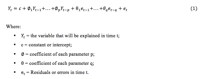
Fava and Vasconcelos (2000) complement that the ARIMA models result from the combination of three components: the auto-regressive component (AR), the integration component (I) and the moving averages component (MA). The model can be adjusted by combining the three components or any subset of them. Thus, an ARIMA model without seasonality can be classified as an ARIMA (p,d,q) (Nau, 2004), where:
• p = the number of autoregressive parameters;
• d = the number of involved differences;
• q = the number of errors/residuals caused by lagged predicting.
The ARIMA model is given by equation 1:
3.2 Exponential smoothing
The exponential smoothing method consists in decomposing the series into components (trend and seasonality) and softening its previous values, i.e., applying different weights whose values decline exponentially to zero for older data, therefore, focusing on the most recent data (Souza et. al. 2008). These exponential smoothing models can also be divided into two groups: additive and multiplicative. In additive models, the amplitude of the seasonal variation is constant over time, i.e., the difference between the highest and lowest value within stations remains relatively constant over time. In multiplicative models, the amplitude of the seasonal variation grows over time (Silva et. al. 2002).
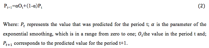
The simple exponential smoothing (SES) was the first exponential smoothing method to be created. According to Souza et. al. (2008) this method is suitable for series that do not have a tendency or seasonality. The formula may be expressed by equation 2:
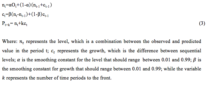
In situations in which the data presents a trend, but does not exhibit seasonality Holt (1957) expanded the simple exponential smoothing and began using two components to conduct the forecast: level and growth. Thus, the formula for the method can be expressed by the following equations:
 Posteriorly, Winters (1960) developed the Holt-Winters method, working with data with trend and seasonality. The method has two forms, one with additive seasonality and another with multiplicative seasonality.
3.3 Criteria for model selection
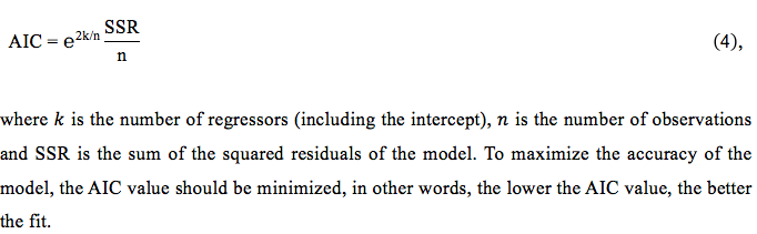
Akaike Information Criterion (AIC) is one of the most important criteria for autoregressive model selection. The great advantage of the AIC is that it imposes a penalty for adding a regressor to the model and works with a kind of tradeoff between the quality of the adjustment of the model and its complexity. According to Gujarati (2006), the AIC can be used to analyze the accuracy of forecast models in and out of the sample, as well as nested and non-nested ones. The AIC can be calculated with equation 4:
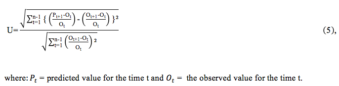
Theil's U can be considered a very important measurement for forecasting, because it can demonstrate if the forecasting result is better or worse than the naive forecast (Hyndman, Koehler, 2006).
For a model to be accepted, the Theil's U should be in a range between zero and one. This is because if the model goes above one, the naive forecast would be more appropriate for the model. The calculation for determining the Theil's U can be done by using equation 5:
4. Research methodology
4.1. Survey data
The data was obtained from the Dow Jones (Dow Jones, 2013) website and corresponds to the Dow Jones Sustainability Index (DJSI) for the period from August 2008 to July 2013. To quantify the forecasting error, quotations from August 2013 to January 2014 were stored.
4.2 Forecasting methods
Two forecasting models were used to find the best forecast: ARIMA and Exponential Smoothing. To generate the forecasting models and result analysis, the "tseries" (Trapletti et. al. 2013) and "forecast" (Hyndman et. al. 2013) packages of the software R (R Core Team, 2013) were used. The most appropriate models for the series were chosen automatically. To automatically approximate an ARIMA model, we used the function auto.arima(), which provide the best ARIMA model according to the information criteria AIC, AICc (AIC correction for small samples) or BIC (Bayesian Information Criterion). The need to apply difference is determined by the R. Confidence intervals of 95% were used for the forecasting. For the exponential smoothing model, we used the function ets(), which selects the best model and estimates the coefficients as needed.
For the ARIMA models, was obtained the best classification to ARIMA (p,d,q); For the exponential smoothing models, we have the terminology ETS (error, trend, seasonality), which may be additive (A), multiplicative (M) or none (N). For example, ETS(A,N,N) is simple exponential smoothing with additive errors.
To determine the best model among those studied, the results of AIC, Theil's U, ACF (autocorrelation function) and PACF (partial autocorrelation function) were analyzed. The best method was determined by the lowest AIC, given that it attains a Theil's U lower than one.
4.3. Residuals tests
After identifying the model and estimating the forecast, a fundamental analysis is to know if the obtained model can properly describe the data. Based on the assumptions that the residuals should follow a normal distribution, they should not be auto correlated, and should present stationarity. After choosing the best model, the tests presented in Table 1 were applied to determine if the model is valid.
| Test | Basic assumption | Null Hypothesis |
| Shapiro-Wilk | Waste normality | Waste that follows the normal distribution |
| Box-Pierce | Waste autocorrelation | Waste that is not correlated |
| Ljung-Box | Waste autocorrelation | Waste that is not correlated |
| White | Homoscedasticity | Residuals that do not exhibit heteroscedasticity |
| Augmented Dickey-Fuller | Stationarity | Unit Root |
Considering a confidence interval of 95%: for the model to be approved in the tests, it must
have a p-value above 0.05 in the Shapiro-Wilk, Box-Pierce, and Ljung-Box tests; for that the null hypothesis not being rejected; and a p-value below 0.05 for the Augmented Dickey-Fuller, so that will be possible to reject the null hypothesis of nonstationary.
5. Results and discussion
The results are presented in two steps: (1) a descriptive analysis of the DJSI time series and comparison between the two models for forecasting and selecting the most suitable one; (2) results of the analysis regarding the best model chosen in step 1 and forecast.
5.1 Data series
The data series presented an average of 1,253.29 points, median of 1,266.65 points, standard deviation of 187.63 points and amplitude of 810.83 points. By analyzing the series, it is clear that there is no seasonality.Figure 1 presents the data series of the DJSI as well as the ACF and PACF correlograms. It is noted by the representation of the series that there was a sharp decline in the indexes from August 2008 until February 2009, and they began to increase again after this period. Furthermore, in 2013 the index presented the best performance in the period studied. The ACF and PACF graphs indicate the autocorrelation between Y and Yt-1 and the autocorrelation between the residuals.
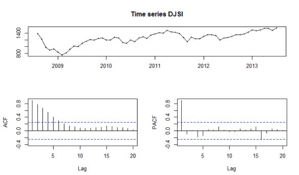
Figure 1. DJSI data series and ACF and PACF correlograms.
While the sharp drop in the index between August 2008 and February 2009 is possibly related to the subprime crisis and the Lehman Brothers bank bankruptcy, this study does not intend to seek causes for the rise or fall in prices of the index.
The naive model does not use statistical methods or prior analysis to gain greater knowledge about the data, it uses the minimum amount of information necessary to determine the forecast for the following periods. The forecast for a step ahead uses the last observed value as the current forecast, even simple, is often the most appropriate, in situations related to the exchange rate and financial market (Souza et. al. 2008). The adjustment for forecast using the naive model produced an AIC = 679.97, which is less than the DJSI forecast by exponential smoothing and higher than that of the ARIMA model.
Tables 2 and 3 present the results of analyses of ARIMA and exponential smoothing models.
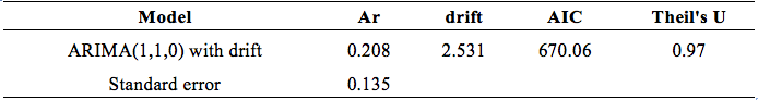
Table 2. Results of the ARIMA model
----
Table 3. Results for the exponential smoothing models
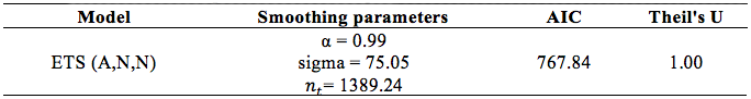
Tables 2 and 3 present the best model selected automatically by the software according to each case. They also present the estimated coefficients, standard error, the AIC and the Theil's U, which are calculated using data within the sample.
Comparing the results of the ARIMA models with exponential smoothing and naive models, we note that the most appropriate model is the ARIMA (1,1,0), since the model has the lowest AIC and still has a Theil's U that is lower than 1. Thus, the selected model will be detailed below, along with the residuals tests for validity of the model.
5.2 Forecast and analysis of the best model
The results demonstrated that the most appropriate model is an ARIMA (1,1,0) which means that the model has an autoregressive component (AR = 0.209) and an integration component (I), i. e., it was necessary to differentiate the series to make it stationary. Thus, the model of this study can be designed from equation 6:
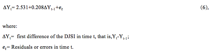
This model presented AIC of 679.55 and Theil's U of 0.97, which is more suitable for forecasting than the naive model, and which is a good result, since the data deal with rates and, in this case, is difficult to forecast.
Figure 2 presents ACF, PACF and residuals charts after making the series stationary, showing that it has no autocorrelation, there is no specific pattern and no significant autocorrelation, indicating the adequacy of the model.
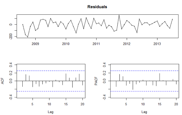
'Figure 2. ACF and PACF of the residuals.
To test the assumptions of the ARIMA model and validate it, some tests were applied. The autocorrelation of residuals was examined using the Box-Pierce tests, which had a p-value of 0.773 and the Ljung-Box test, which had a p-value of 0.677. To test the normality of the residuals, the Shapiro-Wilk presented a p-value of 0.455. In relation to homoscedasticity, the White's test showed a result of 0.207. These results show there is no evidence that would require rejecting the null hypothesis. The augmented Dickey-Fuller test had a value of 0.012 indicating that there is evidence that requires rejection of the null hypothesis (unit root) and thus accept the alternative hypothesis that the series is stationary. Therefore, since it met all the assumptions, we have a valid model for conducting a forecast for a range of 12 months.
Figure 3 shows the data series (the black line) and the predicted values within the sample (the red line). In blue, there is the forecast for the range of 12 months (out of sample). The dark shaded region shows prediction intervals of 80%. The light shaded region presents prediction intervals of 95%, i.e., each future value should be within this shaded region with a probability of 0.95.
Figure 3. Forecast for the DJSI quote by ARIMA (1,1,0).
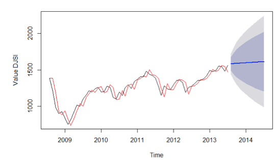
Table 4 presents the predicted values for a range of one year and the higher limits (Hi) and the lower limits (Lo) of 95%. Moreover, it presents the observed and predicted values from August 2013 to February 2014 and the forecasting error obtained using the ARIMA model for DJSI.
Table 4. Predicted Values, confidence interval of 95%, observed values and forecasting error
| Month | Forecast |
Lo 95 |
Hi 95 |
Observed |
Forecasting error |
Aug/13 |
1,581.825 |
1,435.356 |
1,728.295 |
1,536.22 |
-45.605 (-2.97%) |
Sep/13 |
1,587.625 |
1,357.973 |
1,817.277 |
1,623.44 |
35.815 (2.21%) |
Oct/13 |
1,590.835 |
1,297.066 |
1,884.604 |
1,696.6 |
105.765 (6.23%) |
Nov/13 |
1,593.507 |
1,246.603 |
1,940.412 |
1,716.97 |
123.463 (7.19%) |
Dec/13 |
1,596.067 |
1,203.021 |
1,989.114 |
1,733.82 |
137.753 (7.95%) |
Jan/14 |
1,598.605 |
1,164.267 |
2,032.942 |
1,669.91 |
71.305 (4.27%) |
Feb/14 |
1,601.137 |
1,129.102 |
2,073.172 |
1,764.50 |
163.363 (9.26%) |
Mar/14 |
1,603.668 |
1,096.73 |
2,110.607 |
1,783.50 |
179.832 (10.08%) |
Apr/14 |
1,606.20 |
1,066.611 |
2,145.788 |
1,814.37 |
208.170 (11.47%) |
May/14 |
1,608.731 |
1,038.358 |
2,179.103 |
1,841.59 |
232.859 (12.64%) |
Jun/14 |
1,611.262 |
1,011.684 |
2,210.84 |
1,869.62 |
258.358 (13.81%) |
Jul/14 |
1,613.793 |
986.367 |
2,241.219 |
1,840.64 |
226.847 (12.32%) |
The forecast shows that the value of DJSI for the coming months is likely to increase. This result shows that according to the model, those who invest in a portfolio of stocks with the same composition as the DJSI will have a positive outcome. Moreover, it is interesting to analyze that with a confidence interval of 95%, in July 2014 the index should reach a value between 986 and 2,241 points.
This forecast can be useful to investors not only to know index behavior, but also for analyzing what would be the limit of a gain or loss within a certain prediction interval. For example, beginning with the assumption that the DJSI finished the month of July 2013 with a price of 1,563 points. If an investor bought a stock portfolio with the same composition as the index and holds it until July 2014, this investor should have a return of between -36.9% and 41.2% in the period, with a prediction interval of 95%. This provides better risk management for investors.
We can observe in Table 4 that in the first two months (August and September) smaller forecasting errors occurred, -2.97% and 2.21% respectively. This means that the forecast for August overestimated the actual value, unlike that of September, which was underestimated. In other months, the forecast underestimated actual values. To date, the month of December has generated greater forecast error (9.26%). Furthermore, we note that all values are concentrated within the limits of forecast of 95%. Therefore, there is evidence that the model is suitable for predicting future values of the DJSI. The model that best adjustment the data obtained a mean absolute percentage error (MAPE) equal to 4.95%.
6. Conclusion
This study sought to compare the ARIMA and Exponential Smoothing models as tools to predict the future behavior of the Dow Jones Sustainability Index (DJSI) in a range of 12 months. We used the following forecasting methods: Exponential Smoothing, ARIMA and naive. The study used monthly data for the period between August 2008 and July 2013 taken from the Dow Jones (Dow Jones, 2013) website. The best method was chosen based on Theil's U and the AIC criteria. The results found that in the period that was studied the best model was the ARIMA with a Theil's U of 0.97 and AIC of 670.06. The model selected was the ARIMA (1,1,0) with drift, i.e., one autoregressive parameter and the first difference. Based on the residual tests, this model was validated.
The forecasting results indicated that the index, which finished the month of July 2013 at the level of 1,563 points, should close the month of July 2014 between 986.367 points and 2,241.points with a prediction interval of 95%. Furthermore, they demonstrate that the DJSI index is more likely to rise than fall in the 12-month period after July 2013. However, by comparing the values observed to date we note that there was a small drop in the index between July and August 2013 and December 2013 and January 2014. The forecasts always underestimated actual values, except for August 2013, meaning the forecast is conservative and that investors will have a margin of safety for their decision making and thus be able to optimize their investment portfolio.
Among the study's limitations, it is important to note that the DJSI has a behavior that is difficult to predict, because there are numerous factors that can affect the results of the index. However, this study did not seek to deeply study the composition of the index or the criteria used to select the companies, which are based on a specific methodology used by RobecoSam Sustainability Investing. As a suggestion for further research, it is recommended to study in detail the composition of the index and conduct the regression including other explanatory variables such as Gross Domestic Product, exchange rate risk, credit risk and other stock indexes. This would allow using a more robust model, such as regression with panel data.
Acknowledgements
This study is supported by the Coordination for the Improvement of Personnel of Superior Level (Coordenação de Aperfeiçoamento de Pessoal de Nível Superior – CAPES) and National Council for Scientific and Technological Development (Conselho Nacional de Desenvolvimento Científico e Tecnológico – CNPq), Brazil.
References
ABDULLAH, S.; Sapii, N.; Dir, S.; Jalal, T. M. T. (2012); Application of univariate forecasting models of tuberculosis cases in Kelantan. International Conference on Statistics in Science, Business, and Engineering (ICSSBE), Langkawi, Kedah, Malaysia.
ADAMS, C.; Zutshi, A. (2004); Corporate social responsibility: why business should act responsibly and be accountable, Australian Accounting Review, 14(34), 31-39.
ARTIACH, T.; Lee, D.; Nelson, D.; Walker, J. (2010); The determinants of corporate sustainability performance, Accounting & Finance, 50(1), 31-51.
BANCO DO BRASIL (2012); BB ingressa na carteira do índice Dow Jones de Sustentabilidade. Retrieved from http://www.bb.com.br/portalbb/page118,3366,3367,1,0,1,0.bb?codigoNoticia=34965. Accessed on abr. 2014.
BLACKROCK (2014); What is an ETF? A great way to help you meet your goals. Retrieved from http://www.ishares.com/us/education/what-is-an-etf. Accessed on May. 2014
BOX, G. E.; Jenkins, G. M. (1976); Time series analysis, control, and forecasting; San Francisco, Holden-Day, 575 p.
CERIN, P.; Dobers, P. (2001); What does the performance of the Dow Jones Sustainability Group Index tell us? Eco-Management and Auditing, 8(3), 123-133.
CONSOLANDI, C.; Jaiswal-Dale, A.; Poggiani, E.; Vercelli, A. (2009); Global standards and ethical stock indexes: The case of the Dow Jones Sustainability Stoxx Index, Journal of Business Ethics, 87(1), 185-197.
CHATTERJI, A. K.; Levine, D. I.; Toffel, M. W. (2009); How well do social ratings actually measure corporate social responsibility? Journal of Economics & Management Strategy, 18(1), 125-169.
CUNHA, F. A. F. de S.; Samanez, C. P. (2014); Análise de desempenho dos investimentos sustentáveis no mercado acionário brasileiro, Production, 24(2), 420-434.
DILLENBURG, S.; Greene, T.; Erekson, O. H. (2003); Approaching socially responsible investment with a comprehensive ratings scheme: Total social impact, Journal of Business Ethics, 43(3), 167-177.
DOW JONES (2013); Dow Jones Sustainability Indices – in colaboration with RebecoSAM. Retrieved from http://www.sustainability-indices.com. Accessed on jul. 2013.
EDP (2013); Grupo EDP. Retrieved from http://www.edp.pt/pt/sustentabilidade/abordagemasustentabilidade/reconhecimento/dowjonessustainabilityindex/Pages/DowJones.aspx. Accessed on sep. 2013.
FAVA, V. L.; Vasconcelos, M. A. (2000); Manual de econometria; São Paulo, Atlas.
GUJARATI, D. N. (2006); Econometria básica; Rio de Janeiro, Elsevier, 817 p.
HOLT, C. (1957); Forecasting trends and seasonal by exponentially weighted averages. Carnegie Institute of Technology, Pittsburg, PA.
HYNDMAN, R. J.; Athanasopoulos, G. (2013); Forecasting: principles and practice. Melbourne, Australia: OTexts. Retrieved from http://www.otexts.com/fpp/. Accessed on sep. 2013.
HYNDMAN, R. J.; Koehler, A. B. (2006); Another look at measures of forecast accuracy, International Journal of Forecasting, 22(4), 679-688.
HYNDMAN, R.J.; Razbash, S.; Schmidt, D. (2012); Forecast: Forecasting functions for time series and linear models. R package version, v. 3.
KANG, H. H.; Liu, S. B. (2014); Corporate social responsibility and corporate performance: a quantile regression approach, Quality & Quantity, 48(6), 3311-3325.
KNOEPFEL, I. (2001); Dow Jones Sustainability Group Index: a global benchmark for corporate sustainability, Corporate Environmental Strategy, 8(1), 6-15.
LÓPEZ, M. V.; Garcia, A.; Rodriguez, L. (2007); Sustainable development and corporate performance: A study based on the Dow Jones sustainability index, Journal of Business Ethics, 75(3), 285-300.
MACHADO, M. R.; Machado, M. A. V.; Corrar, L. J. (2009); Desempenho do Índice de Sustentabilidade Empresarial (ISE) da bolsa de valores de São Paulo, Revista Universo Contábil, FURB, 5(2), 24-38.
MARTINS, V. L. M.; Werner, L. (2014); Comparação de previsões individuais e suas combinações: um estudo com séries industriais, Production, 24(3), 618-627.
NAU, R. F. (2004); Decision 411: forecasting. Fuqua School of Business, Duke University.
O'ROURKE, A. (2003); The message and methods of ethical investment, Journal of Cleaner Production, 11(6), 683-693.
R CORE TEAM. (2013); R: A language and environment for statistical computing. R Foundation for Statistical Computing, Vienna, Austria. Retrieved from http://www.R-project.org/. Accessed on aug. 2013.
ROBINSON, M.; Kleffner, A.; Bertels, S. (2011); Signaling sustainability leadership: empirical evidence of the value of DJSI membership, Journal of Business Ethics, 101(3), 493–505.
SADOWSKI, M.; Whitaker, K.; Buckingham, F. (2010); Rate the Raters: Phase One e Look Back and Current State. Sustainability, London, UK.
SALZMANN, O.; Somers, A.; Steger, U. (2005); The business case for corporate sustainability: literature review and research options, European Management Journal, 23(1), 27-36.
SEARCY, C.; Elkhawas, D. (2012); Corporate sustainability ratings: An investigation into how corporations use the Dow Jones Sustainability Index, Journal of Cleaner Production, 35, 79-92.
SILVA, W. V. da; Samohyl, R. W.; Costa, L. S. (2002); Comparação entre os métodos de previsão univariados para o preço médio da soja no Brasil. XXII Encontro Nacional de Engenharia de Produção, Curitiba, PR, Brazil.
SINGH, E. H. (2013); Forecasting Tourist Inflow in Bhutan using Seasonal ARIMA, International Journal of Science and Research, 2(9), 242-245.
SOUZA, G. P.; Samohyl, R. W.; Miranda, R. G. D. (2008); Métodos simplificados de previsão empresarial; Rio de Janeiro, Editora Ciência Moderna, 181 p.
SPARKES, R.; Cowton, C. J. (2004); The maturing of socially responsible investment: a review of the developing link with corporate social responsibility, Journal of Business Ethics, 52(1), 45-57.
TRAPLETTI, A.; Hornik, K.; Lebaron, B. (2013); Time series analysis and computational finance. Package: tseries, Version: 0.10-32.
TRIERWEILLER, A. C.; Peixe, B. C. S.; Tezza, R.; Bornia, A. C.; Campos, L. M. S. (2013); Measuring environmental management disclosure in industries in Brazil with Item Response Theory, Journal of Cleaner Production, 47, 298-305.
VONDRA, T.; Sedivy, J. (2013); Maximizing Utilization in Private IaaS Clouds with Heterogenous Load through Time Series Forecasting, International Journal on Advances in Systems and Measurements, 6(1 and 2), 149-165.
WERNER, L.; Ribeiro, J. L. D. (2003); Previsão de demanda: uma aplicação dos modelos Box-Jenkins na área de assistência técnica de computadores pessoais, Revista Gestão & Produção, 10(1), 47-67.
WINTERS, P. R. (1960); Forecasting sales by exponentially weighted moving averages, Management Science, 6(3), 324-342.
1. Doutoranda em Engenharia de Produção na Universidade Federal de Santa Catarina. Pesquisa temas: Teoria de Resposta ao Item, psicometria, construção de instrumentos de medida e testes adaptativos computadorizados. Graduada em Matemática pela Universidade de Passo Fundo, mestre em Modelagem Computacional pela Universidade Federal do Rio Grande. Production Engineering Department, Santa Catarina Federal University (UFSC), Brazil. Email: debospenassato@gmail.com
2. Pesquisadora Pós-doutoranda do Programa de Pós Graduação em Engenharia de Produção da Universidade Federal de Santa Catarina (UFSC), pesquisa o uso da Teoria da Resposta ao Item, em temas relacionados à área ambiental e estratégia organizacional. É Doutora (2010), Mestre (2004) e Especialista (2000) em Engenharia de Produção, Bacharel em Administração (1993), todos pela UFSC. Pesquisadora na área ambiental e de inovação. Production Engineering Department, Santa Catarina Federal University (UFSC), Brazil. Email: andreatri@gmail.com
3. Professor titular da Universidade Federal de Santa Catarina (UFSC). Tem experiência na área de Engenharia de Produção, com ênfase em Análise de Custos e aplicações da Teoria da Resposta ao Item. Possui graduação em Engenharia Mecânica pela Universidade Federal do Paraná (1985), Mestrado (1988) e Doutorado (1995), ambos em Engenharia de Produção pela UFSC. Production Engineering Department, Santa Catarina Federal University (UFSC), Brazil. Email: cezar.bornia@ufsc.br
4. Doutorando em Engenharia de Produção (UFSC). Mestre em Engenharia da Produção (UFSM). Economista (UFSM). Atuou durante seis anos no mercado financeiro, onde trabalhou para corretoras de valores do Brasil atuando na captação e acompanhamento de investimentos para pessoas físicas, e ministrou diversas palestras e cursos sobre o mercado de capitais. É integrante do Laboratório de Custos e Medidas (LCM/UFSC), também colabora com o Núcleo de Gestão Empresarial (NGE/UFSM). Tem experiência na área de Economia, com ênfase em Mercado de Capitais, Finanças Corporativas, Planejamento Estratégico, Análise de Investimentos, Avaliação de Desempenho, Custos e Aplicações Empresariais da Teoria da Resposta ao Item. Production Engineering Department, Santa Catarina Federal University (UFSC), Brazil. Email: lorenzofrazzon@yahoo.com